
The 4th Set of Nets: Rotational Riemann-sum Visualization
Loading the math board and drawing, please wait…
In collections
How many nets of a cuboid are there?
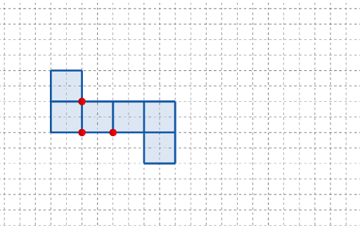
This example demonstrates a rotational construction of the 4th “net” (grid-like polygon arrangement) to visually connect structured geometry with sum-based approximations, resembling upper and lower Riemann sums. It emphasizes core ideas such as upper/lower sum (Riemann-sum intuition), linear functions and their angle/geometry relationships, and a broader viewpoint linking summation behavior to probability & random processes (including hypergeometric distribution as referenced by the topic tags). In GeoGebra, the construction is built using Point, Polygon, and Rotate: key points (A, B, C, and parameter-driven points like q1, q2, q4, q5, q6 with t) define polygonal regions, while Rotate generates rotated copies (q4', q2', q5', q6'_1, t') to form the next set. Interactive controls (button1, button2) and annotations (text1) support stepwise comparison of different nets. Suitable for advanced middle school through early university, especially for teaching geometric constructions, transformations, and the visual approach to integration via Riemann sums.
GeoGebra Commands & Parameters
Point(Ray[(1, 0), (3, 0)]) → APoint(Ray[A + (1, 0), A + (2, 0)]) → CPoint(Ray[A + (0, 1), A + (0, 2)]) → BPolygon({(0, 0), A, B, (0, y(B))}) → q1Polygon({A, C, (x(C), y(B)), B}) → q2Polygon({B, B + (0, h), B + ((-l), h), B + ((-l), 0)}) → q4Polygon({C, C + (l, 0), C + (l, w), C + (0, w)}) → q5Polygon({C + (l, 0), C + (l + h, 0), C + (l + h, w), C + (l, w)}) → q6Rotate(q4, (90° * t), Line[(0, w), B]) → q4'Rotate(q2, (90° * t), Line[B, A]) → q2'Rotate(Rotate[q5, (90° * t), Line[C + (0, w), C]], (90° * t), Line[B, A]) → q5'Rotate(Rotate[Rotate[q6, (90° * t), Line[C + (l, w), C + (l, 0)]], (90° * t), Line[C + (0, w), C]], (90° * t), Line[B, A]) → q6'_{1}Polygon({C + (l, 0), C + (l, (-l)), C + (l + h, (-l)), C + (l + h, 0)}) → q3Rotate(Rotate[Rotate[Rotate[q3, (90° * t), Line[C + (l + h, 0), C + (l, 0)]], (90° * t), Line[C + (l, w), C + (l, 0)]], (90° * t), Line[C + (0, w), C]], (90° * t), Line[B, A]) → q3'
AI Drawing Prompt Reference
Draw a rotational grid structure composed of multiple polygons to illustrate the connection between geometric shapes and sum-based approximations. Start by creating a rectangular frame, then form four polygonal regions inside it, one in each corner. Next, rotate these polygons around the center of the frame to generate copies at different angles. Finally, combine these rotated polygons to create a complex, layered grid structure that visually demonstrates the concept of upper and lower Riemann sums.
The prompt above was compiled from the original drawing commands and is for reference only.