
Zeros of Polynomial Functions by BHNmath
Loading the math board and drawing, please wait…
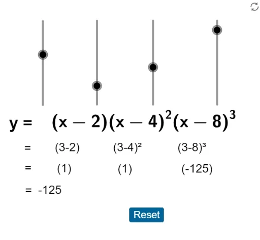
This example demonstrates the distribution of zeros and the changes in the graph of polynomial functions. Key math concepts include polynomial functions, zeros, and function graph transformations. GeoGebra commands/objects used include l, q, m, c, b, a, d, g, e, h, i, p, j, f, A, text2, text5, text6, text7, text8, text9, text3, text4, text10, k, text11, Point (dependent), text1, text13, text14, text15, button1, text16, n, text12 for function definition, graph drawing, and interactive demonstration. Suitable for high school mathematics teaching to understand the properties and transformation rules of polynomial functions.
GeoGebra Commands & Parameters
Numeric l(1)q(x) = If[-5 ≤ x ≤ -1 ∨ 1 ≤ x ≤ 5, x, 1]q(l)Numeric c(8)Numeric b(4)Numeric a(2)Numeric d(3)g(x) = x - ag(d)h(x) = (x - b)^(2)h(d)p(x) = (x - c)^(3)p(d)f(x) = If[x ≥ 0, (((m * (x - a)) * (x - b)^(2)) * (x - c)^(3))](d, f(d))f(d)Point Point (dependent)(NaN, NaN, NaN)true
AI Drawing Prompt Reference
Draw the distribution of zeros and graph transformations of polynomial functions. First, show a piecewise constant function, then calculate and plot multiple transformed functions based on it, including linear, quadratic, and cubic transformations, marking key points to demonstrate the zero distribution and graph changes of polynomial functions.
The prompt above was compiled from the original drawing commands and is for reference only.