
Wulff Canvas: Building Wulff-Type Geometry via Sphere–Plane Intersections
Loading the math board and drawing, please wait…
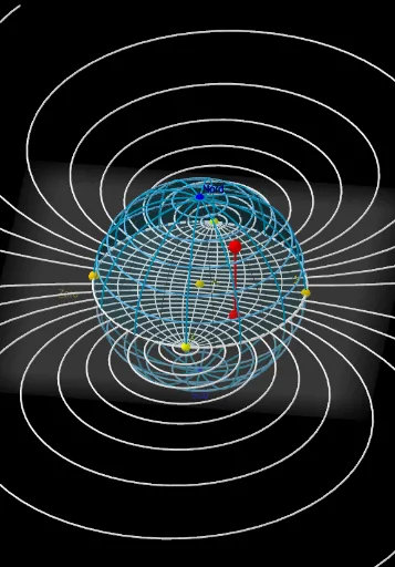
This example demonstrates how a Wulff-canvas style construction can be visualized by intersecting a sphere with a family of planes to obtain structured curves (e.g., circle arcs/paths) and the resulting geometric layout. The key math ideas include solid geometry (sphere, plane, and intersection loci), circle and circumcircle arcs as building blocks, and centroid/barycenter-inspired reference positioning through orthogonality and projection-like steps. In GeoGebra, the construction uses Sequence to generate parameter sets, Sphere to create the 3D carrier surface, Plane plus OrthogonalPlane to define cutting planes in controlled directions, and OrthogonalLine for perpendicular reference geometry. Intersect and IntersectPath compute intersection points/paths, while PointIn, Point, and Ray ensure intersection events are selected on the intended regions. Finally, CircumcircleArc, Circle, and Element are used to assemble and display the circle/arc components that form the Wulff canvas visualization. Suitable for high school advanced geometry, early undergraduate geometric construction, and STEM visualization/modeling lessons.
GeoGebra Commands & Parameters
Sequence(Circle[(0, 1 / sin((k * π / ((2 * n_B))))), sqrt(1 / sin((k * π / ((2 * n_B))))^(2) - 1)], k, (-n_B), n_B) → cercles1Sequence(CurveCartesian[(cos(φ) * sin(λ) / (1 + (cos(φ) * cos(λ)))), sin(φ) / (1 + (cos(φ) * cos(λ))), φ, -1.5708, 1.5708], λ, -1.5707963267948966, 1.5707963267948966, π / ((2 * n_L))) → Cercles2Sphere(M, Nord) → aPlane(M, Nord, Zero) → bIntersectPath(b, a) → cIntersectPath(xOyPlane, a) → dOrthogonalPlane(Nord, xAxis) → eIntersectPath(e, a) → fPointIn(a) → PPlane(P, Nord, M) → gIntersectPath(g, a) → hOrthogonalPlane(P, zAxis) → iIntersectPath(i, a) → kRay(Zero, P) → jIntersect(j, e) → P'Segment(Zero, B) → lPoint(l) → WCircumcircleArc(Zero, Nord, B) → pPoint(cercles1) → ASegment(P, A) → mSequence(CurveCartesian[x(M) + (cos(i) * cos(j)), y(M) + (cos(i) * sin(j)), z(M) + sin(i), i, 0, π / 2], j, 0, (2 * π), (2 * π / 8)) → l1Sequence(CurveCartesian[x(M) + (cos(i) * cos(j)), y(M) + (cos(i) * sin(j)), z(M) + sin(i), j, 0, (2 * π)], i, 0, (2 * π), π / 12) → l2PointIn(a) → CSegment(C, A) → nElement(l2, 1) → oCircle((0.018164476916503913, 0.003027412819417208), 1) → qCircle((0, 0), 1) → rOrthogonalLine(C, s) → tIntersect(t, s) → ESurface(x(M) + (cos(i) * cos(j)), y(M) + (cos(i) * sin(j)), z(M) + sin(i), i, 0, π, j, 0, π) → uSegment(C, E) → f_1Sequence(CurveCartesian[x(M) + (cos(i) * cos(j)), y(M) + (cos(i) * sin(j)), z(M) + sin(i), i, 0, (2 * π)], j, 0, π, (2 * π / 12)) → l3
AI Drawing Prompt Reference
Visualize a Wulff-canvas style geometry by intersecting a sphere with a family of planes to create structured curves like circular arcs and paths, revealing the geometric layout. Start with a sphere as the carrier surface, generate a sequence of parameterized circles, and intersect them with various planes. Use orthogonal planes and projection-like steps to position key points, then assemble circular arcs and circles to form the Wulff canvas visualization.
The prompt above was compiled from the original drawing commands and is for reference only.