
Writing Equations to Represent Tables 003: Random Generation and Interactive Ver
Loading the math board and drawing, please wait…
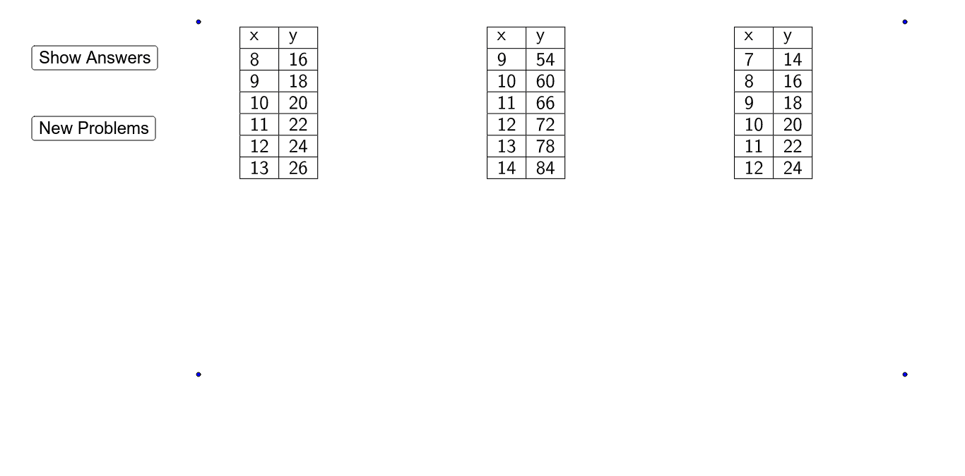
This GeoGebra example demonstrates how to convert tabular data into linear equations through an interactive interface, with random generation and answer-checking features. The core mathematical concept is representing a linear function in the form y = mx + b by analyzing the relationship between x and y values in a table. The construction uses the Random command to generate starting values and coefficients, the If command to control answer display buttons, and the TableText command to present data in a table format. Multiple objects such as button1, button2, StartingX1, coefficientX1, and ShowAnswers are employed to manage user input and feedback. This resource is suitable for middle and high school students learning functions and equations, as well as for teachers demonstrating the connection between tables, equations, and graphs in a classroom setting.
GeoGebra Commands & Parameters
Random(1, 10) → StartingX1Random(1, 10) → StartingX2Random(1, 10) → StartingX3Random(1, 10) → StartingX4Random(1, 10) → StartingX5Random(1, 10) → StartingX6Random(1, 10) → coefficientX1Random(1, 10) → coefficientX2Random(1, 10) → coefficientX3Random(1, 10) → coefficientX4Random(1, 10) → coefficientX5Random(1, 10) → coefficientX6If(ShowAnswers ≟ true, (("y = " * coefficientX1) * "x"), "y") → yLabel1If(ShowAnswers ≟ true, (("y = " * coefficientX2) * "x"), "y") → yLabel2If(ShowAnswers ≟ true, (("y = " * coefficientX3) * "x"), "y") → yLabel3If(ShowAnswers ≟ true, (("y = " * coefficientX4) * "x"), "y") → yLabel4If(ShowAnswers ≟ true, (("y = " * coefficientX5) * "x"), "y") → yLabel5If(ShowAnswers ≟ true, (("y = " * coefficientX6) * "x"), "y") → yLabel6TableText({{A1, B1}, {A2, B2}, {A3, B3}, {A4, B4}, {A5, B5}, {A6, B6}, {A7, B7}}, "|_") → Table1TableText({{D1, E1}, {D2, E2}, {D3, E3}, {D4, E4}, {D5, E5}, {D6, E6}, {D7, E7}}, "|_") → Table2TableText({{G1, H1}, {G2, H2}, {G3, H3}, {G4, H4}, {G5, H5}, {G6, H6}, {G7, H7}}, "|_") → Table3TableText({{J1, K1}, {J2, K2}, {J3, K3}, {J4, K4}, {J5, K5}, {J6, K6}, {J7, K7}}, "|_") → Table4TableText({{M1, N1}, {M2, N2}, {M3, N3}, {M4, N4}, {M5, N5}, {M6, N6}, {M7, N7}}, "|_") → Table5TableText({{P1, Q1}, {P2, Q2}, {P3, Q3}, {P4, Q4}, {P5, Q5}, {P6, Q6}, {P7, Q7}}, "|_") → Table6
AI Drawing Prompt Reference
Draw a graph that includes six linear equation labels, each displayed as y = mx + b. Also include six tables, each with seven rows of data. The construction order should be: first create the six equation labels, then create the six tables. Ensure the labels and tables are clear and visible to understand the relationship between linear functions and tabular data.
The prompt above was compiled from the original drawing commands and is for reference only.