
Why the Derivative of Sine is Cosine?
Loading the math board and drawing, please wait…
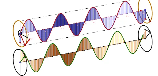
This GeoGebra example dynamically illustrates why the derivative of the sine function equals the cosine function. By constructing a circle, tangent lines, and rotating vectors, it visually connects the geometric slope of the tangent to the analytical concept of a derivative. Core mathematical concepts include trigonometric functions, differentiation, circular motion, and vector geometry. The construction employs GeoGebra commands such as Circle, Tangent, Intersect, Vector, Sequence, and CurveCartesian to animate the tangent's direction and trace its locus. The example is suitable for calculus classrooms, high school advanced mathematics, or anyone exploring the relationship between trigonometry and differential calculus.
GeoGebra Commands & Parameters
Circle(O, R, xAxis) → cRotate(A, (-t), xAxis) → A'Segment(O, A') → fTranslate(c, Vector[O, B]) → c'Segment(C, O') → gSegment(D, O') → hSequence((i, 0, (R * sin(i))), i, 0, t - (4 * π), (2 * π / Step)) → l1Sequence((i, 0, 0), i, 0, t - (4 * π), (2 * π / Step)) → l2Sequence(Segment[Element[l1, i], Element[l2, i]], i, 1, Length[l1]) → l3Segment(O, E) → iSegment(O - (0, 0, R), O + (0, 0, R)) → jSegment(A', E) → kSegment(E, O) → lMidpoint(O, A) → FMidpoint(O, F) → GMidpoint(A', O) → HMidpoint(H, O) → IRotate(G, ((-t)) / 2, xAxis) → G'CircumcircleArc(G, G', I) → eSegment(O, A) → mRotate(G, t / 2, xAxis) → G'_1CircumcircleArc(G, G'_1, I) → pSegment(D, C) → n_1Tangent(A', c) → n,Circle(A', R, xAxis) → qIntersect(n, q) → J, KVector(A', K) → uCircle(A', R, xAxis) → rPoint(zAxis) → LVector(A', L) → vTranslate(K, Vector[(If[t < 0.5, 0, If[0.5 < t < (4 * π), t / 15, 1]] * v)]) → K'CurveCartesian(i, 0, (R * sin(i)), i, 0, t - (4 * π)) → aCurveCartesian(i, 0, R, i, 0, t - (4 * π)) → bCurveCartesian(i, 0, (-R), i, 0, t - (4 * π)) → dTranslate(r, Vector[(If[t < 0.5, 0, If[0.5 < t < (4 * π), t / 15, 1]] * v)]) → r'Translate(A', Vector[(If[t < 0.5, 0, If[0.5 < t < (4 * π), t / 15, 1]] * v)]) → A''Vector(A'', K') → wRay(L, L + (1, 0, 0)) → sCurveCartesian(i, 0, (R * cos(i)), i, 0, t - (4 * π)) → oTranslate(o, Vector[O, L]) → o'Circle(M, R, s) → c_1Segment(M, N) → f_1Segment(P, M) → g_1Segment(P, N) → h_1Vector(L, L + ((15 * π / 2), 0, 0)) → u_1Sequence(Translate[L, Vector[(i * u_1)]], i, 0, 1, 1 / 15) → l4Segment(L - (0, 0, R), O + (0, 0, R)) → i_1Sequence(L + (i, 0, (R * cos(i))), i, 0, t - (4 * π), (2 * π / Step)) → l5Sequence(L + (i, 0, 0), i, 0, t - (4 * π), (2 * π / Step)) → l6Sequence(Segment[Element[l5, i], Element[l6, i]], i, 1, Length[l5]) → l7
AI Drawing Prompt Reference
Create a dynamic illustration showing why the derivative of the sine function equals the cosine function. Draw a circle and mark a point on it, then draw the tangent line at that point. Rotate the point around the circle to show the changing direction of the tangent line and trace the path of its endpoint. Use vectors to represent the tangent direction and connect it to the cosine function's graph. The visualization should dynamically demonstrate the relationship between the derivative of sine and cosine, suitable for mathematical education.
The prompt above was compiled from the original drawing commands and is for reference only.