
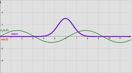
Wave Equation Demonstration
Loading the math board and drawing, please wait…
In collections
UQ-Applied Mathematical Analysis
This example demonstrates the graphical representation of solutions to the wave equation under given boundary conditions. It involves core mathematical concepts such as Fourier series, trigonometric functions, sequence summation, and polygon construction. Key GeoGebra commands/objects used include Sequence, Sum, Polygon, and Textfield. Suitable for high school and above students to learn and understand mathematical modeling of wave phenomena.
GeoGebra Commands & Parameters
Sequence((2 / L * Integral[(f(x) * sin((((π * x) * i)) / L)), 0, L]), i, 1, n) → AnSequence((2 / (((i * π) * a)) * Integral[(g(x) * sin((((π * x) * i)) / L)), 0, L]), i, 1, n) → BnSequence(((Element[An, i] * cos((((i * π) * a) * y / L))) * sin(((i * π) * x / L))), i, 1, n) → AnCSSequence(((Element[Bn, i] * sin((((i * π) * a) * y / L))) * sin(((i * π) * x / L))), i, 1, n) → BnSSSequence(Element[AnCS, i] + Element[BnSS, i], i, 1, n) → AnBnSum(AnBn, n) → uPolygon((xmin1, -0.5), (-0.05, -0.5), (-0.05, 0.5), (xmin1, 0.5)) → Range1, h, i, j, kPolygon((xmin2, ymin2), (L, ymin2), (L, ymax2), (xmax2, ymax2)) → Range2, l, m, p, qTextfield(f0) → InputBox1Textfield(g0) → InputBox2Textfield(L) → InputBox3Textfield(a) → InputBox4Textfield(n) → InputBox5