Wallace–Simson Theorem Construction

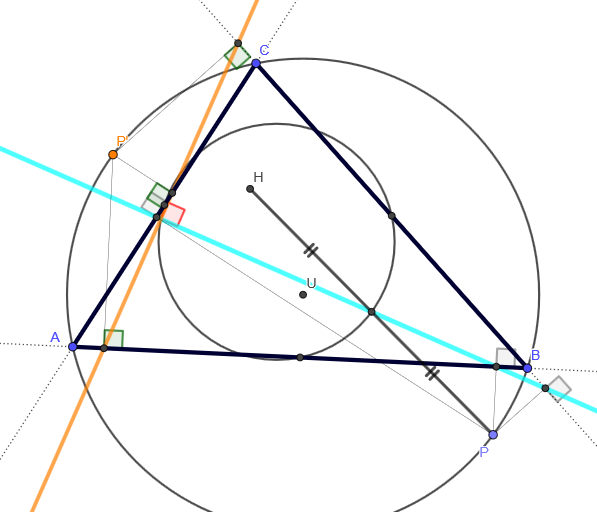
This GeoGebra example demonstrates the Wallace–Simson (Wallace–Simson) theorem: for a point moving on the circumcircle of a triangle, the perpendicular feet (or the corresponding perpendicular lines) produce a collinear configuration, revealing a stable linear relationship tied to the triangle–circle structure. Key concepts include a triangle’s circumcircle, perpendicular lines and feet, circle–line intersections, and angle relations that underpin the theorem. Construction highlights: Polygon builds the base triangle; Line and Segment create sides and auxiliary segments; Midpoint and Center determine key reference points such as the circumcenter; Circle defines the circumcircle; Intersect is used to obtain intersection points between lines and the circle; OrthogonalLine constructs the perpendiculars whose feet are the main data points; Angle is used to mark/control angle constraints; and Mirror is employed to generate symmetric points/lines (e.g., producing a reflected counterpart such as P′). It uses points representing the triangle vertices (A, B, C), circumcircle-related centers and intersections, the perpendicular-foot points, and mirrored points. Suitable for high-school geometry exploration and for classroom demonstrations of theorem verification in dynamic geometry settings.