
Volumes of Solids with Different Cross Sections
Loading the math board and drawing, please wait…
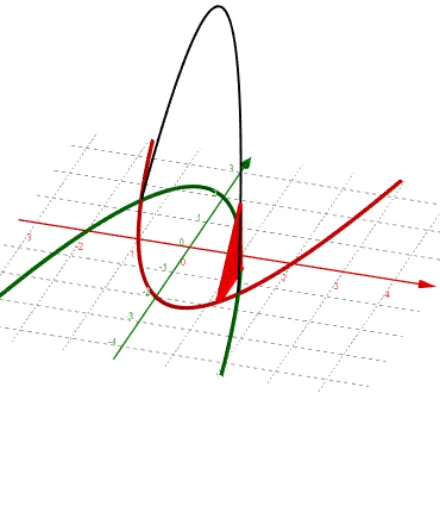
This example demonstrates how to visualize and calculate the volume of solids with varying cross sections. It involves core math concepts like volume calculation, right triangles, trigonometry, similar triangles, and solid geometry. GeoGebra commands such as Segment, Point, Polygon, and IntegralBetween are used in the construction. Suitable for high school students and math enthusiasts exploring 3D geometry volume methods.
GeoGebra Commands & Parameters
SelectedElement(C) → text1IndexOf(text1, C) → aIntersect(f, g, 1) → AIntersect(f, g, 2) → BSegment((x(A), -3), (x(B), -3)) → hPoint(h) → DSegment(E, F) → iCurveCartesian(t, g(t), p(t), t, x(A), x(B)) → bCurveCartesian(t, f(t), p(t), t, x(A), x(B)) → cPolygon(E, F, (x(F), f(x(F)), p(x(F))), (x(F), g(x(F)), p(x(F)))) → q1, e, f_1, j, kSurface(t, g(t), (u * p(t)), t, x(A), x(B), u, 0, 1) → dSurface(t, f(t), (u * p(t)), t, x(A), x(B), u, 0, 1) → lSurface(t, (u * g(t)) + ((1 - u) * f(t)), p(t), t, x(A), x(B), u, 0, 1) → mPolygon(E, F, F + (0, 0, e), E + (0, 0, e)) → q2, e_1, f_2, n, qCurveCartesian(t, g(t), f(t) - g(t), t, x(A), x(B)) → oCurveCartesian(t, f(t), f(t) - g(t), t, x(A), x(B)) → rSurface(t, g(t), (u * (f(t) - g(t))), t, x(A), x(B), u, 0, 1) → sSurface(t, f(t), (u * (f(t) - g(t))), t, x(A), x(B), u, 0, 1) → tSurface(t, (u * f(t)) + ((1 - u) * g(t)), f(t) - g(t), t, x(A), x(B), u, 0, 1) → uMidpoint(i) → GSurface(t, ((f(t) - g(t)) / 2 * cos(u)) + (f(t) + g(t)) / 2, ((f(t) - g(t)) / 2 * sin(u)), t, x(A), x(B), u, 0, (2 * π)) → vOrthogonalPlane(G, i) → wPointIn(w) → HLine(G, H) → g_1Circle(G, (f(x(G)) - g(x(G))) / 2, g_1) → c_1IntegralBetween(f, g, x(A), x(B)) → a_1CurveCartesian(t, (f(t) + g(t)) / 2, ((f(t) - g(t)) / 2 * sqrt(3)), t, x(A), x(B)) → bbSurface(t, (u * g(t)) + ((1 - u) * y(bb(t))), ((1 - u) * z(bb(t))), t, x(A), x(B), u, 0, 1) → b_1Surface(t, (u * f(t)) + ((1 - u) * y(bb(t))), ((1 - u) * z(bb(t))), t, x(A), x(B), u, 0, 1) → d_1Rotate(Polygon[E, F, 3], π / 2, e) → t1CurveCartesian(t, f(t), f(t) - g(t), t, x(A), x(B)) → hhPolygon(E, F, F + (0, 0, f(x(F)) - g(x(F)))) → t2, i_1, e_2, f_3Surface(t, (u * g(t)) + ((1 - u) * f(t)), ((1 - u) * z(hh(t))), t, x(A), x(B), u, 0, 1) → h_1Surface(t, f(t), (u * z(hh(t))), t, x(A), x(B), u, 0, 1) → j_1Surface(t, ((f(t) - g(t)) / 2 * cos(u)) + (f(t) + g(t)) / 2, ((f(t) - g(t)) / 2 * sin(u)), t, x(A), x(B), u, 0, π) → k_1Rotate(Semicircle[E, F], π / 2, e) → p_1
AI Drawing Prompt Reference
Draw a solid with varying cross-sections. First, plot two curves f and g. Then, create a series of rectangular cross-sections parallel to the x-axis between these curves. Use these cross-sections to construct the solid surface. Finally, calculate and display the volume enclosed by the two curves.
The prompt above was compiled from the original drawing commands and is for reference only.