
Cones, Statistics, and Isosceles Triangles
Loading the math board and drawing, please wait…
In collections
geometriadinamica.es
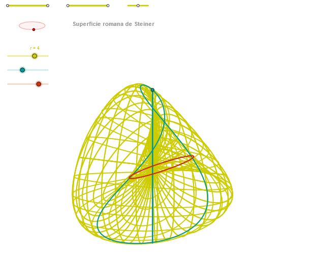
This example demonstrates the geometric relationships between cones, statistical data, and isosceles triangles. It involves core concepts like cone sections, statistical analysis, and the orthocenter of isosceles triangles. Construction highlights include using commands such as Segment, Point, OrthogonalLine, Circle, Intersect, Ellipse, Angle, CurveCartesian, and Sequence. Suitable for high school mathematics education, focusing on the integration of solid geometry and analytical geometry.
GeoGebra Commands & Parameters
Segment(Q3, Q4) → p2Point(p2) → P3Segment(P3, Q4) → p4Point(p4) → P4Segment(Q1, Q2) → p1Point(p1) → P1Segment(P1, Q2) → p3Point(p3) → P2OrthogonalLine(C, xAxis) → zz2Circle(C, 0.62) → zz0Intersect(zz0, zz2, 1) → ZZ4Intersect(zz0, zz2, 2) → ZZ3Ellipse(ZZ3, ZZ4, 0.65) → zElipse2Point(zElipse2) → ZIntersect(zElipse2, zz2) → ZZ7, ZZ8Angle(ZZ8, C, Z) → zAngIncOrthogonalLine(C, yAxis) → zz1Intersect(zz0, zz1, 2) → ZZ2Intersect(zz0, zz1, 1) → ZZ1Ellipse(ZZ1, ZZ2, 0.65) → zElipse1Point(zElipse1) → XYIntersect(zElipse1, zz1) → ZZ5, ZZ6Angle(ZZ6, C, XY) → zAngRotSegment(Q5, Q6) → p5Point(p5) → P5Segment(ZZ5, ZZ6) → zz4Segment(ZZ7, ZZ8) → zz3Intersect(zElipse2, zElipse1, 1) → zPunto1Intersect(zElipse2, zElipse1, 4) → zPunto2Segment(zPunto1, zPunto2) → zSeg2CurveCartesian((r * (((sin((2 * v)) * (cos(α))^(2)) * sin(zAngRot)) + ((sin(v) * sin((2 * α))) * cos(zAngRot)))), (r * (((((-sin((2 * v))) * (cos(α))^(2)) * cos(zAngRot)) * sin(zAngInc)) + (((sin(v) * sin((2 * α))) * sin(zAngRot)) * sin(zAngInc)) + ((cos(v) * sin((2 * α))) * cos(zAngInc)))), v, v1, v2) → curva2CurveCartesian(0, (r * ((-sin((2 * u))) * cos(zAngInc))), u, u1, u2) → curva1CurveCartesian((r * (((sin((2 * β)) * (cos(u))^(2)) * sin(zAngRot)) + ((sin(β) * sin((2 * u))) * cos(zAngRot)))), (r * (((((-sin((2 * β))) * (cos(u))^(2)) * cos(zAngRot)) * sin(zAngInc)) + (((sin(β) * sin((2 * u))) * sin(zAngRot)) * sin(zAngInc)) + ((cos(β) * sin((2 * u))) * cos(zAngInc)))), u, u1, u2) → a1Sequence(CurveCartesian[(r * (((sin((2 * v)) * (cos(u))^(2)) * sin(zAngRot)) + ((sin(v) * sin((2 * u))) * cos(zAngRot)))), (r * (((((-sin((2 * v))) * (cos(u))^(2)) * cos(zAngRot)) * sin(zAngInc)) + (((sin(v) * sin((2 * u))) * sin(zAngRot)) * sin(zAngInc)) + ((cos(v) * sin((2 * u))) * cos(zAngInc)))), v, v1, v2], u, u1, u2, (2 * paso)) → list2Sequence(CurveCartesian[(r * (((sin((2 * v)) * (cos(u))^(2)) * sin(zAngRot)) + ((sin(v) * sin((2 * u))) * cos(zAngRot)))), (r * (((((-sin((2 * v))) * (cos(u))^(2)) * cos(zAngRot)) * sin(zAngInc)) + (((sin(v) * sin((2 * u))) * sin(zAngRot)) * sin(zAngInc)) + ((cos(v) * sin((2 * u))) * cos(zAngInc)))), u, u1, u2], v, v1, v2, paso) → list1
AI Drawing Prompt Reference
Draw a graph that includes cone sections, statistical data, and isosceles triangles. The graph should have the cone's axis, ellipses, angles, and curves. The construction order should include drawing the axis, circles, ellipses, intersection points, angle calculations, and curve drawing.
The prompt above was compiled from the original drawing commands and is for reference only.