Volumes of Revolution: Disk and Washer Method Demonstration

Loading the math board and drawing, please wait…

2012-07-21 22:59

In collections Calculus Concepts

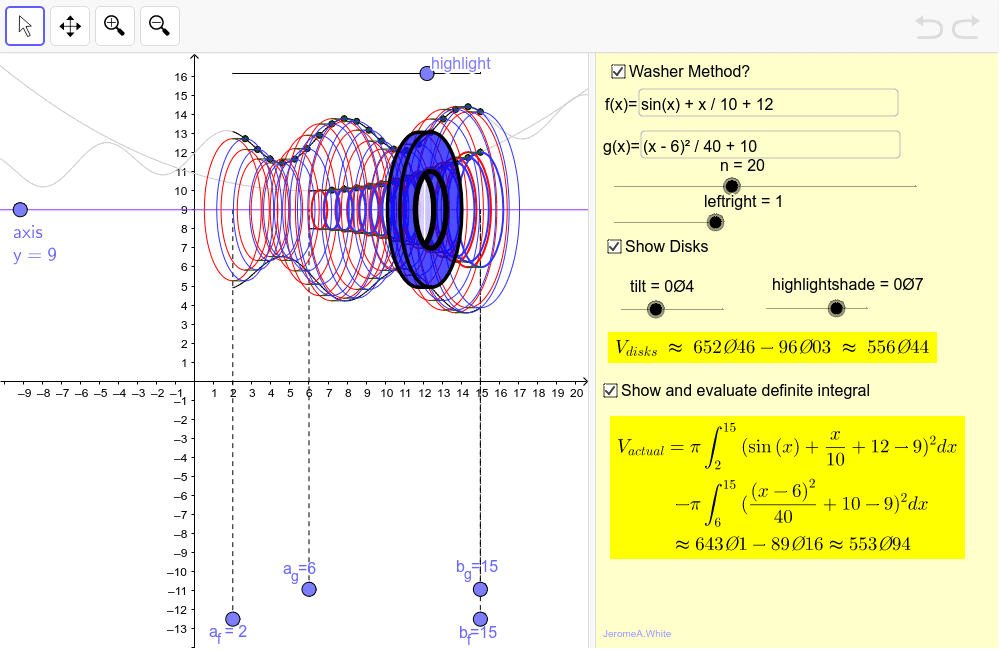
This GeoGebra example demonstrates the disk and washer method for computing volumes of solids of revolution using definite integrals. It dynamically visualizes how a plane region bounded by functions f and g rotates around a coordinate axis to generate a solid, with cross-sectional disks or washers whose volumes are approximated by Riemann sums and compared to the exact integral value. Core mathematical concepts include definite integration, the disk method, the washer method, volume of revolution, functions, limits of integration, and solid geometry. The construction employs GeoGebra commands such as Point, Segment, Sequence, Function, Mirror, Textfield, Integral, Translate, Corner, Element, CurveCartesian, Circle, Intersect, and Polygon, together with objects like sliders n, sliderYoffset, offsetYaxis, sliderXoffset, offsetXaxis, Δx, function f and g, axis, listf_{radii}, Vf_{approx}, and Vf_{actual}. It is suitable for high school calculus electives, undergraduate mathematical analysis, and engineering mathematics courses, as well as self-study of geometric applications of definite integrals and three-dimensional volume computation.

GeoGebra Commands & Parameters

Point(offsetYaxis) → axis
Point(offsetXaxis) → a_f
Point(offsetXaxis) → b_f
Segment(a_f + (0, sliderXoffset2), b_f + (0, sliderXoffset2)) → innerslider
Point(innerslider) → a_g
Point(innerslider) → b_g
Sequence((af_x + i, axis_y), i, 0, Δx * (n - 1), Δx) → list_{centers}
Sequence((af_x + i + leftright * Δx, f(af_x + i + leftright * Δx)), i, 0, Δx * (n - 1), Δx) → listf_{points}
Sequence(If[(x(Element[list_{centers}, i]) < ag_x) ∨ (x(Element[list_{centers}, i]) > bg_x - Δx), Corner[1] + (-1, -1), (x(Element[listf_{points}, i]), g(x(Element[listf_{points}, i])))], i, 1, n) → listg_{points}
Function(f, af_x, bf_x) → f_1
Sequence(abs(y(Element[listf_{points}, i]) - y(Element[list_{centers}, i])), i, 1, n) → listf_{radii}
Sequence((0, Element[listf_{radii}, i] * sqrt(1 - tilt^(2))), i, 1, n) → listf_c
Sequence(Ellipse[Element[listf_{foci1}, i], Element[listf_{foci2}, i], Element[listf_{radii}, i]], i, 1, n) → listf_{ellipses1}
Sequence(Segment[Element[listf_{points}, i] - (leftright * Δx, 0), Element[listf_{points}, i] + ((1 - leftright) * Δx, 0)], i, 1, n) → listf_{segments1}
Mirror(listf_{segments1}, axisline) → listf_{segments2}
Textfield(f) → inputBox1
Integral(π * (f(x) - axis_y)^(2), af_x, bf_x) → Vf_{actual}
Segment(a_f, (af_x, axis_y)) → segment_a
Segment(b_f, (bf_x, axis_y)) → segment_b
Sequence(If[(x(Element[list_{centers}, i]) < ag_x) ∨ (x(Element[list_{centers}, i]) > bg_x - Δx), 0, abs(y(Element[listg_{points}, i]) - y(Element[list_{centers}, i]))], i, 1, n) → listg_{radii}
Function(g, ag_x, bg_x) → g_1
Sequence((0, Element[listg_{radii}, i] * sqrt(1 - tilt^(2))), i, 1, n) → listg_c
Sequence(Ellipse[Element[listg_{foci1}, i], Element[listg_{foci2}, i], Element[listg_{radii}, i]], i, 1, n) → listg_{ellipses1}
Textfield(g) → inputBox2
Translate(listf_{ellipses1}, Vector[(0, 0), (Δx, 0)]) → listf_{ellipses2}
Translate(listg_{ellipses1}, Vector[(0, 0), (Δx, 0)]) → listg_{ellipses2}
Sequence(Segment[Element[listg_{points}, i] - (leftright * Δx, 0), Element[listg_{points}, i] + ((1 - leftright) * Δx, 0)], i, 1, n) → listg_{segments1}
Mirror(listg_{segments1}, axisline) → listg_{segments2}
Integral(π * (g(x) - axis_y)^(2), ag_x, bg_x) → Vg_{actual}
Corner(6) → A
Segment(a_g, (ag_x, axis_y)) → segmenti_a
Segment(b_g, (bg_x, axis_y)) → segmenti_b
Segment((x(a_f), sliderXoffset3), (x(b_f), sliderXoffset3)) → ellipseslider
Point(ellipseslider) → highlight
Element(list_{centers}, ellipsenumber) → ellipsecenter
Element(listf_{radii}, ellipsenumber) → ellipsef_a
Element(listf_{ellipses2}, ellipsenumber) → ellipsef
CurveCartesian(x(ellipsecenter) + ellipsef_b * cos(t), y(ellipsecenter) + ellipsef_a * sin(t), t, 1.5707963267948966, 4.71238898038469) → ellipsehalf1_f
Element(listf_{segments1}, ellipsenumber) → segmentf1
Element(listf_{segments2}, ellipsenumber) → segmentf2
Element(listg_{ellipses2}, ellipsenumber) → ellipseg
Element(listg_{radii}, ellipsenumber) → ellipseg_a
Circle((0, 0), ellipseg_a) → d
Circle((Δx / tilt, 0), ellipseg_a) → e
Intersect(d, e) → B, C, ,
CurveCartesian(x(ellipsecenter) + ellipseg_b * cos(t), y(ellipsecenter) + ellipseg_a * sin(t), t, -β, β) → ellipsepart_g
CurveCartesian(x(ellipsecenter) + Δx + ellipsef_b * cos(t), y(ellipsecenter) + ellipsef_a * sin(t), t, 1.5708, 4.71238898038469) → ellipsehalf2_f
CurveCartesian(x(ellipsecenter) + Δx + ellipsef_b * cos(t), y(ellipsecenter) + ellipsef_a * sin(t), t, -1.5708, 1.5707963267948966) → ellipsehalf3_f
Polygon({(0, ellipsef_a), (Δx, ellipsef_a), (Δx, -ellipsef_a), (0, -ellipsef_a)} + ellipsecenter) → poly1, , , ,
Function(-f(x) + 2 * axis_y, af_x, bf_x) → f_2
Function(-g(x) + 2 * axis_y, ag_x, bg_x) → g_2
CurveCartesian(x(ellipsecenter) + Δx + ellipseg_b * cos(t), y(ellipsecenter) + ellipseg_a * sin(t), t, π - β, π + β) → ellipsepartb_g

AI Drawing Prompt Reference

Draw a planar region bounded by two adjustable curves f(x) and g(x) that rotates around a horizontal axis to illustrate the disk and washer methods for volumes of revolution. Show the axis, a set of equally spaced vertical slices whose number, axis offset, and slice width Δx are controlled by sliders. Each slice produces a disk (radius from f to the axis) or a washer (inner radius from g, outer from f). Display the elliptical cross‑sections of the slices, their mirrored edge segments, the Riemann‑sum approximation of the volume, and the exact integral values for both functions.

The prompt above was compiled from the original drawing commands and is for reference only.