
Cylindrical Shell Action!!! (2) – Dynamic Volume of Revolution
Loading the math board and drawing, please wait…
In collections
BC Calculus
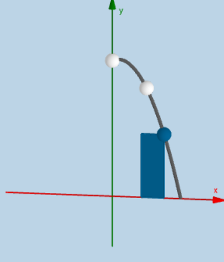
① This interactive GeoGebra example dynamically illustrates the volume of a solid of revolution using the method of cylindrical shells, allowing users to visualize how thin cylindrical shells approximate the total volume. ② The core mathematical concept is the shell method for computing volumes of revolution, based on the integral formula V = 2π∫ x·f(x) dx, involving functions, rotation, and the limit of Riemann sums. ③ The construction uses GeoGebra commands such as Point, Polynomial, Integral, Sequence, Polygon, Line, Surface, Vector, Cylinder, Rotate, Dilate, and Segment, creating objects like the function f, axis of rotation, partition intervals, shell sequence (list1, poly1), and the rotated surfacescars. A slider n controls the number of shells, enabling dynamic exploration of the approximation process. ④ This resource is suitable for high school calculus or introductory college calculus courses, serving as a visual aid for teachers or as an interactive tool for students to understand the shell method and volume integration.
GeoGebra Commands & Parameters
Point(x = 0) → APoint(x = 2) → BPoint(x = 4) → CPolynomial({A, B, C}) → fIntegral(h, x(A), x(C)) → aPoint(h) → DSequence(Polygon[((i * deltax), 0), (((i + 1) * deltax), 0), (((i + 1) * deltax), h(((i + 1) * deltax))), ((i * deltax), h(((i + 1) * deltax)))], i, 0, n - 1, 1) → list1Polygon(D, (x(D) - deltax, y(D)), (x(D) - deltax, 0), (x(D), 0)) → poly1, d, i, j, kLine(E, F) → lSurface((t * cos(u)), h(x(D)), (t * sin(u)), t, x(D) - deltax, x(D), u, 0, α) → eVector(D, (x(D), 0, 0)) → uSurface((t * cos(u)), 0, (t * sin(u)), t, x(D) - deltax, x(D), u, 0, α) → mCylinder((0, 0, 0), (0, y(D), 0), x(D)) → o, p, q, rCylinder((0, 0, 0), (0, y(D), 0), x(D) - deltax) → s, t, c_1, vSurface((t * cos(u)), h(t), (t * sin(u)), t, 0, 10, u, 0, α) → bRotate(list1, (-α), l) → list1'Rotate(poly1, (-α), l) → poly1'Dilate(G, If[0 < w ≤ 1, 1 - w, 0], D) → G'Segment(G, G') → f_1Rotate(D, π, l) → D'Rotate((x(D) - deltax, y(D)), π, l) → JDilate(H, If[1 < w ≤ 2, 2 - w, 0], I) → H'Segment(H, H') → g_1Dilate(D', If[2 < w ≤ 3, 3 - w, 0], J) → J'Segment(D', J') → i_1Rotate(h, (-α), l) → h_1
AI Drawing Prompt Reference
Draw a solid of revolution around the y-axis of a function f(x) fitted through points A(0,0), B(2,0), and C(4,0). Use a dynamic method to approximate the volume of the solid with a sequence of thin cylindrical shells, where the radius of each shell goes from the x-axis to the value of f(x), and the height is dx. Observe how the approximation improves as the number of shells n increases.
The prompt above was compiled from the original drawing commands and is for reference only.