
Volume of Rotation via Riemann Sums: Midpoint Approximation
Loading the math board and drawing, please wait…
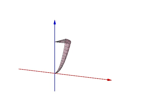
This example demonstrates how to approximate the volume of a solid of revolution using Riemann sums, showing how the estimate improves as the number of subintervals increases. It centers on the idea of computing volume by summing cross-sectional areas (the disk method) and approximating integrals with midpoint values on each interval. Key concepts include volume of rotation, the Riemann-sum framework, and midpoint approximation for numerical integration. In the GeoGebra construction, commands such as If are used for conditional, piecewise control of objects, Surface is used to generate the rotated 3D geometry, and Sequence is used to build the subdivision/index sequences (controlled by parameters like n/nn) that drive the approximation. The constructed objects (including parameters for radii/section heights such as r, function-related items such as f and g, and multiple interval/length elements like l1–l14) collectively build the rotating solid and its volume estimate. Suitable for high school to early university calculus lessons and interactive modeling with GeoGebra.
GeoGebra Commands & Parameters
If(a < 10, 1, If[a < 20, 2, If[a < 30, 4, If[a < 40, 5, If[a < 50, 8, 4]]]]) → nnIf(a < 10, a, If[a < 20, a - 10, If[a < 30, a - 20, If[a < 40, a - 30, If[a < 50, a - 40, If[a < 60, a - 50, If[a < 70, a - 60, If[a < 80, a - 70, If[a < 90, a - 80, a - 90]]]]]]]]) → bSurface((r * cos(t)), (r * sin(t)), r^(2), r, 0, 2, t, 0, (b * 0.63)) → cSurface((r * cos(t)), (r * sin(t)), 4, r, 0, 2, t, 0, (b * 0.63)) → dSurface((r * cos(t)), (r * sin(t)), 1, r, 0, 1, t, 0, (b * 0.63)) → eSequence(Surface[(u * cos(t)), (u * sin(t)), ((m - 1) * 4 / nn), u, 0, sqrt(((m - 1) * 4 / nn)), t, 0, (b * 0.63)], m, 1, nn) → l2Sequence(Surface[(sqrt((4 * (m - 1) / nn)) * cos(t)), (sin(t) * sqrt((4 * (m - 1) / nn))), z, z, (4 * (m - 1) / nn), (4 * m / nn), t, 0, (b * 0.63)], m, 1, nn) → l1Sequence(Surface[u, 0, z, u, 0, sqrt((4 * (m - 1) / nn)), z, ((m - 1) * 4 / nn), (m * 4 / nn)], m, 1, nn) → l3Sequence(Surface[(u * cos((b * 0.63))), (u * sin((b * 0.63))), z, u, 0, sqrt((4 * (m - 1) / nn)), z, ((m - 1) * 4 / nn), (m * 4 / nn)], m, 1, nn) → l4Surface(u, 0, z, z, 1, 1 + dd, u, 0, 1) → hSurface((r * cos(t)), (r * sin(t)), 1 + dd, r, 0, 1, t, 0, (b * 0.63)) → fSurface(cos(t), sin(t), z, z, 1, 1 + dd, t, 0, (b * 0.63)) → gSurface((r * cos((b * 0.63))), (r * sin((b * 0.63))), z, r, 0, 1, z, 1, 1.2) → iSequence(Surface[u, 0, z, u, (2 * (m - 1) / nn), (2 * m / nn), z, 0, ((2 * (m - 1) / nn))^(2)], m, 1, nn) → l5Sequence(Surface[u, ((((m - 1) * 2 / nn))^(2) * sin(t)), ((((m - 1) * 2 / nn))^(2) * cos(t)), u, ((m - 1) * 2 / nn), (m * 2 / nn), t, 0, (b * 0.63)], m, 1, nn) → l7Sequence(Surface[u, (r * sin((b * 0.63))), (r * cos((b * 0.63))), u, (2 * (m - 1) / nn), (2 * m / nn), r, 0, ((2 * (m - 1) / nn))^(2)], m, 1, nn) → l6Surface(u, (u^(2) * sin(t)), (u^(2) * cos(t)), u, 0, 2, t, 0, (b * 0.63)) → jSequence(Surface[((m - 1) * 2 / nn), (r * sin(t)), (r * cos(t)), r, 0, (((m - 1) * 2 / nn))^(2), t, 0, (b * 0.63)], m, 1, nn) → l8Surface(2, (r * sin(t)), (r * cos(t)), r, 0, 4, t, 0, (b * 0.63)) → kSurface(u, ((1 - u^(2)) * sin(t - 3.14)), 1 + ((1 - u^(2)) * cos(t - 3.14)), u, 0, 1, t, 0, (0.63 * b)) → lSurface(0, (r * sin(t - 3.14)), 1 + (r * cos(t - 3.14)), r, 0, 1, t, 0, (b * 0.63)) → mSurface(u, 0, If[z > u^(2), z], u, 0, 1, z, 0, 1) → oSurface(u, If[r > u^(2), ((1 - r) * sin((b * 0.63) - 3.14))], If[r > u^(2), 1 + ((1 - r) * cos((b * 0.63) - 3.14))], u, 0, 1, r, 0, 1) → pSequence(Surface[(m * 1 / nn), (r * sin(t - 3.14)), 1 + (r * cos(t - 3.14)), r, 0, 1 - (m / nn)^(2), t, 0, (b * 0.63)], m, 1, nn) → l9Sequence(Surface[u, ((1 - (m / nn)^(2)) * sin(t - 3.14)), 1 + ((1 - (m / nn)^(2)) * cos(t - 3.14)), u, (m - 1) / nn, m / nn, t, 0, (b * 0.63)], m, 1, nn) → l10Surface(2 + ((2 - r) * sin(t - 1.62)), ((2 - r) * cos(t - 1.62)), 0, r, 0, 2, t, 0, (b * 0.63)) → rSurface(2 + ((2 - r) * sin(t - 1.62)), ((2 - r) * cos(t - 1.62)), r^(2), r, 0, 2, t, 0, (b * 0.63)) → qSequence(Surface[2 + (r * sin(t - 1.62)), (r * cos(t - 1.62)), ((4 * m)) / nn, r, 0, 2 - sqrt(((4 * m)) / nn), t, 0, (b * 0.63)], m, 1, nn) → l11Sequence(Surface[2 + ((2 - sqrt(((4 * m)) / nn)) * sin(t - 1.62)), ((2 - sqrt((4 * m / nn))) * cos(t - 1.62)), z, t, 0, (b * 0.62), z, ((m - 1) * 4 / nn), (m * 4 / nn)], m, 1, nn) → l12Surface((r * cos(t)), (r * sin(t)), r^(2), r, 1, 2, t, 0, (b * 0.62)) → sSurface(cos(t), sin(t), z, z, 1, 4, t, 0, (b * 0.62)) → tSurface(u, 0, If[z > u^(2), z], u, 1, 2, z, 1, 4) → uSurface((r * cos((b * 0.62))), (r * sin((b * 0.62))), If[z > r^(2), z], r, 1, 2, z, 1, 4) → vSurface((r * cos(t)), (r * sin(t)), 4, r, 1, 2, t, 0, (b * 0.62)) → wSequence(Surface[(r * cos(t)), (r * sin(t)), 1 + (m * 3 / nn), r, 1, sqrt(1 + (m * 3 / nn)), t, 0, (b * 0.63)], m, 1, nn) → l13Sequence(Surface[(sqrt(1 + ((m - 1) * 3 / nn)) * cos(t)), (sqrt(1 + ((m - 1) * 3 / nn)) * sin(t)), z, t, 0, (b * 0.63), z, 1 + ((m - 1) * 3 / nn), 1 + (m * 3 / nn)], m, 1, nn) → l14Surface((r * cos(t)), (r * sin(t)), r^(2), r, 0, 2, t, 0, (b * 0.63)) → a_1Surface((r * cos(t)), (r * sin(t)), (2 * r), r, 0, 2, t, 0, (b * 0.63)) → b_1Sequence(Surface[u_{1}, 0, z, u_{1}, (2 * sqrt(m / nn)), (2 * sqrt((m + 1) / nn)), z, (4 * m / nn), (4 * (m + 1) / nn)], m, 0, nn - 1) → l15Sequence(Surface[(r * cos(t)), (r * sin(t)), 1 + (m * 3 / nn), r, 0, 1, t, 0, (b * 0.63)], m, 1, nn) → l20Sequence(Surface[cos(t), sin(t), z, t, 0, (b * 0.63), z, 1 + ((m - 1) * 3 / nn), 1 + (m * 3 / nn)], m, 1, nn) → l16Sequence(Surface[u_{1}, 0, z, u_{1}, 0, 1, z, 1 + ((m - 1) * 3 / nn), 1 + (m * 3 / nn)], m, 1, nn) → l17Sequence(Surface[(r * cos((b * 0.62))), (r * sin((b * 0.62))), z, r, 0, 1, z, 1 + (3 * (m - 1) / nn), 1 + (3 * m / nn)], m, 1, nn) → l18
AI Drawing Prompt Reference
Draw a 3D graph of a solid of revolution approximated by Riemann sums. The graph consists of multiple 3D surfaces, each representing an approximate volume element on a subinterval. The construction order is to first create the rotating solid, then generate multiple surfaces via sequences, gradually refining the approximation. Key objects include radius r, number of subintervals n, functions f and g, and surfaces c, d, e. The graph illustrates how the volume estimate improves as the subdivision increases.
The prompt above was compiled from the original drawing commands and is for reference only.