
Visualizing Variance of Two Distributions
Loading the math board and drawing, please wait…
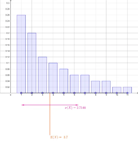
This GeoGebra example dynamically compares the variance of two different distributions, illustrating differences in data dispersion. Core mathematical concepts include mean, variance, standard deviation, and distribution shape. Construction uses Segment and Point to create data points, mean to compute averages, stdevp for population standard deviation, BarChart for histograms, Vector for deviation arrows, and multiple text objects (text1-text7) to label key statistics. Suitable for high school and introductory college statistics, helping students grasp variance as a measure of spread and how distribution shapes affect it.
GeoGebra Commands & Parameters
Segment((1, 0), (11, 0)) → thexaxisPoint(thexaxis) → A12Point(thexaxis) → A13Point(thexaxis) → A14Point(thexaxis) → A15Point(thexaxis) → A16Point(thexaxis) → A17Point(thexaxis) → A18Point(thexaxis) → A19Point(thexaxis) → A20Point(thexaxis) → A21Point(thexaxis) → A22Point(thexaxis) → A23Point(thexaxis) → A24Point(thexaxis) → A25Point(thexaxis) → A26Point(thexaxis) → A27Point(thexaxis) → A28Point(thexaxis) → A29Point(thexaxis) → A30Point(thexaxis) → A31Point(thexaxis) → A32Point(thexaxis) → A33Point(thexaxis) → A34Point(thexaxis) → A35Point(thexaxis) → A36Point(thexaxis) → A37Point(thexaxis) → A38Point(thexaxis) → A39Point(thexaxis) → A40Point(thexaxis) → A41Point(thexaxis) → A42Point(thexaxis) → A43Point(thexaxis) → A44Point(thexaxis) → A45Point(thexaxis) → A46Point(thexaxis) → A47Point(thexaxis) → A48Point(thexaxis) → A49Point(thexaxis) → A50Point(thexaxis) → B13Point(thexaxis) → B14Point(thexaxis) → B15Point(thexaxis) → B16Point(thexaxis) → B17Point(thexaxis) → B18Point(thexaxis) → B19Point(thexaxis) → B20Point(thexaxis) → B21Point(thexaxis) → B22Point(thexaxis) → B23Point(thexaxis) → B24Point(thexaxis) → B25Point(thexaxis) → B26Point(thexaxis) → B27Point(thexaxis) → B28Point(thexaxis) → B29Point(thexaxis) → B30Point(thexaxis) → B31Point(thexaxis) → B32Point(thexaxis) → B33Point(thexaxis) → B34Point(thexaxis) → B35Point(thexaxis) → B36Point(thexaxis) → B37Point(thexaxis) → B38Point(thexaxis) → B39Point(thexaxis) → B40Point(thexaxis) → B41Point(thexaxis) → B42Point(thexaxis) → B43Point(thexaxis) → B44Point(thexaxis) → B45Point(thexaxis) → B46Point(thexaxis) → B47Point(thexaxis) → B48Point(thexaxis) → B49Point(thexaxis) → B50mean(thexs1) → mean1mean(thexs2) → mean2Segment((mean1, (meandepth * ymin)), (mean1, 0)) → meanpos1Segment((mean2, (meandepth * ymin)), (mean2, 0)) → meanpos2Point(thexaxis) → B12BarChart(Sequence[11], freq1, 0.8) → dist1BarChart(Sequence[11], freq2, 0.8) → dist2Point(thexaxis) → A11Point(thexaxis) → B11Point(thexaxis) → A1Point(thexaxis) → A2Point(thexaxis) → A3Point(thexaxis) → A4Point(thexaxis) → A5Point(thexaxis) → A6Point(thexaxis) → A7Point(thexaxis) → A8Point(thexaxis) → A9Point(thexaxis) → A10Point(thexaxis) → B1Point(thexaxis) → B2Point(thexaxis) → B3Point(thexaxis) → B4Point(thexaxis) → B5Point(thexaxis) → B6Point(thexaxis) → B7Point(thexaxis) → B8Point(thexaxis) → B9Point(thexaxis) → B10stdevp(thexs1) → sd1stdevp(thexs2) → sd2Vector((mean1, (sddepth * ymin)), (mean1 - sd1, (sddepth * ymin))) → sdleft1Vector((mean1, (sddepth * ymin)), (mean1 + sd1, (sddepth * ymin))) → sdright1Vector((mean2, (sddepth * ymin)), (mean2 - sd2, (sddepth * ymin))) → sdleft2Vector((mean2, (sddepth * ymin)), (mean2 + sd2, (sddepth * ymin))) → sdright2
AI Drawing Prompt Reference
Draw 50 points on the horizontal axis, then generate two sets of data points based on these 50 points, with 25 points in each set. Represent the distribution of these two sets of data with bar charts, and calculate the mean, standard deviation, and variance for each set. Use arrows to show the deviation of each data point from the mean, and label the mean, standard deviation, and variance for each set with text.
The prompt above was compiled from the original drawing commands and is for reference only.