Visualizing Binomial Distributions for Large Trials

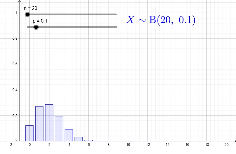
① This example demonstrates the probability distribution of a binomial random variable for large numbers of trials using a bar chart, allowing users to observe how the distribution shape changes with parameters. ② The core mathematical concept is the binomial distribution, including its probability mass function, parameters n (number of trials) and p (success probability), and the tendency toward symmetry as n increases. ③ Construction details: The GeoGebra commands Sequence and BarChart are used to generate trial indices and plot the probability bars; key objects include n, p, thexs (x-axis values), thefreqs (corresponding frequencies), thedist (distribution object), coordinate range variables xmin, xmax, ymin, ymax, and a text label text1 for parameter display. ④ Suitable for high school or college probability and statistics courses, this interactive tool helps students explore binomial distribution properties dynamically and can be used for classroom demonstrations or self-study.