Visualizing Upper and Lower Riemann Sums

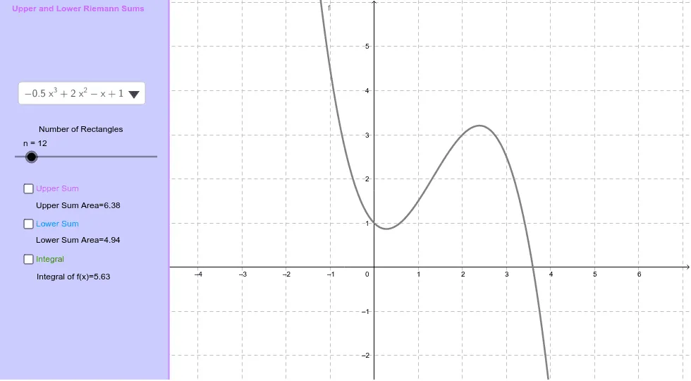
This GeoGebra example dynamically illustrates the upper and lower Riemann sums for a selected function over a given interval, alongside the exact definite integral value, enabling students to intuitively grasp how Riemann sums approximate the integral as the partition refines. Core mathematical concepts include Riemann sums, definite integrals, interval partitioning, function graphing, and the idea of limits. Construction highlights: the SelectedElement command picks the function, UpperSum and LowerSum generate the upper and lower rectangle sums, Integral computes the exact area, and CreatePanel builds an interactive control panel; key objects include function f, endpoints A and B, partition number n, rectangle sum objects UpperSum_1 and LowerSum_1, text labels text1–text5, and polygon poly1. Suitable for high school and early college calculus learners, this resource supports classroom demonstrations or self-study, allowing users to adjust slider n to observe how the upper and lower sums converge to the integral value as the number of subintervals increases.