
Riemann Sums and Integrals by hpp3
Loading the math board and drawing, please wait…
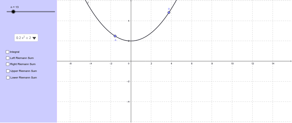
This example illustrates the concepts of Riemann sums and integrals. By adjusting the number of segments, you can observe how Riemann sums approximate the integral value. Key mathematical concepts include integrals, Riemann sums, and their geometric applications. GeoGebra commands used include Function, LeftSum, Integral, and Sequence. Suitable for high school and above students learning calculus.
GeoGebra Commands & Parameters
CreatePanel(240) → poly1, aSelectedElement(Function) → fPoint(f) → APoint(f) → BLeftSum(f, x(A), x(B), n) → LeftSum_1Integral(f, x(A), x(B)) → Integral_1LowerSum(f, x(A), x(B), n) → UpperSum_1LowerSum(f, x(A), x(B), n) → LowerSumSequence(x(A) + (i * dx), i, 0, n) → subintTake(subint, 2, n + 1) → rightTake(subint, 1, n) → leftSequence(Polygon[(Element[left, i], 0), (Element[right, i], 0), (Element[right, i], Element[rightheights, i]), (Element[left, i], Element[rightheights, i])], i, 1, n) → rightRect
AI Drawing Prompt Reference
Draw a function curve and display its left and right Riemann sums and integral. Adjust the number of segments to observe how the sums approximate the integral. Start by plotting the function, then draw rectangles for the left and right Riemann sums below the curve, aligned with the x-axis. Highlight the exact integral area. Arrange all rectangles sequentially from left to right, marking segment points, and show the combined effect of all graphics.
The prompt above was compiled from the original drawing commands and is for reference only.