Visualizing Polynomial Roots and Complex Roots

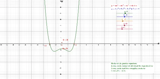
This GeoGebra example dynamically displays the roots of a polynomial (both real and complex) on the complex plane, using equilateral triangles and ratios to aid understanding of root-coefficient relationships. Core mathematical concepts include polynomial root-finding, complex number representation, Vieta's formulas, and the geometric interpretation of roots. Construction highlights: the Root command computes real roots, ComplexRoot computes complex roots, and SurdText displays roots in radical form; objects include the polynomial function f, root points Root_1 to Root_4, complex points z_1 to z_6 with text labels, and auxiliary segments/triangles (g, h, i, j, p). Suitable for high school and above in algebra, complex numbers, or math lab activities, allowing students to observe how roots change as polynomial coefficients vary.