Visualizing Normal Approximation to Binomial with Continuity Correction

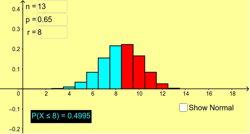
① This interactive GeoGebra example visually demonstrates how the normal distribution approximates the binomial distribution as the number of trials increases, and highlights the need for a continuity correction when matching discrete probabilities to continuous areas. ② Core mathematical concepts include binomial distribution, normal distribution, central limit theorem approximation, continuity correction, probability histograms, and area under density curves. ③ Construction details: The applet uses GeoGebra commands such as BinomialDist to generate binomial probabilities, Sequence to create lists, BarChart for the probability histogram, Normal for the normal density curve, Integral to compute areas under the curve, and Textfield/inputBox1-3 for interactive parameter control (n, p, and correction toggle). Additional objects like Max, Slider, and dynamic text labels support real-time updates. ④ Suitable for high school and introductory college statistics courses, particularly for teaching when the normal approximation is valid (np and n(1-p) > 5) and why continuity correction improves accuracy. It also serves as a tool for exploring approximation error under varying parameters.