
Normal Distribution to Standard Normal Distribution Conversion
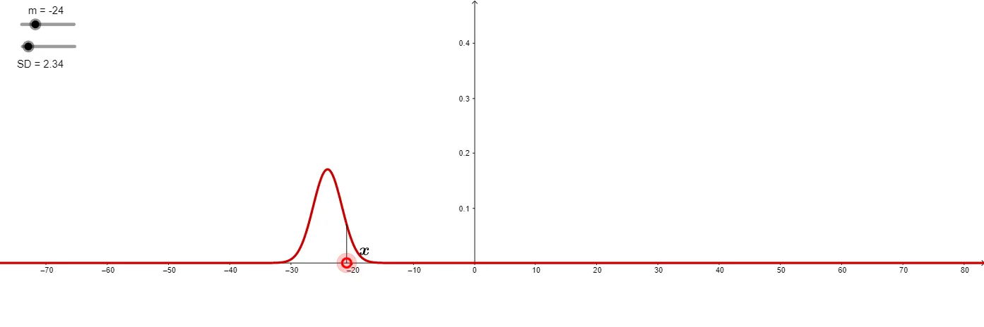
Loading the math board and drawing, please wait…
This GeoGebra example dynamically demonstrates the transformation of a general normal distribution into the standard normal distribution, visually illustrating the geometric meaning of data standardization (z-scores). Core mathematical concepts include the probability density function of the normal distribution, how the mean and standard deviation affect the curve shape, the standard normal distribution (mean 0, standard deviation 1), and the relationship between cumulative probability and integration. Construction highlights: the Normal command generates the normal curve, Point and Segment mark the mean, standard deviation, and data points, Integral computes the area (probability) under the curve, and sliders or text objects link the z-value conversion. Suitable for high school and college statistics courses to understand the standardization formula z=(x-μ)/σ, probability calculations, and distribution symmetry.
GeoGebra Commands & Parameters
Normal(m, SD, x, false) → fPoint(xAxis) → ASegment(B, A) → aIntegral(f, -Infinity, x(A)) → bNormal(0, 1, x, false) → gSegment(C, D) → cIntegral(g, -Infinity, x(C)) → d
AI Drawing Prompt Reference
Draw a normal distribution curve with adjustable mean and standard deviation, and overlay a standard normal distribution curve. Mark a data point on the x-axis, connect it to the mean with a segment to show deviation. Shade the area under the curve to the left of this point to represent cumulative probability. On the standard normal curve, mark the corresponding standardized point, connect it to the origin with a segment, and shade its left area. Use sliders or text to dynamically show the conversion between the original value and the z-score.
The prompt above was compiled from the original drawing commands and is for reference only.