
Visualizing a Parasolic Surface
Loading the math board and drawing, please wait…
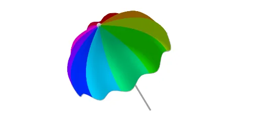
This example demonstrates how to construct and visualize a parasolic surface (a structured curved surface) by assembling geometric elements and generating its shape through a systematic parameter-driven setup. Key mathematics concepts include surface modeling in 3D (Surface), constructing guiding curves/sections, and using midpoint and circle-based geometry to build the surface from discretized elements. From the provided construction summary, the model is built with GeoGebra commands CurveCartesian, Surface, Midpoint, Sequence, Segment, and Circle. It uses base objects/points (e.g., O, P), parameters such as R, amplitude, and frequency-like quantities (c, f), and creates many intermediate points (e.g., A1…A15, B1…B17) that serve as sampled cross-section or control locations; these are then connected/organized to form the final surface via Surface. Suitable for advanced secondary students and early university learners for 3D geometry visualization, geometric construction practice, and introductory surface modeling in STEM education.
GeoGebra Commands & Parameters
CurveCartesian(x(O) + sin((ondes * t)) / amplitude, y(O) + (R * sin(t)), z(O) + (R * cos(t)), t, 0, (3 * π)) → cSurface(x(O) + ((1 - f(v)) * z(c(u))) + (v * z(P)) - 2, y(O) + ((1 - f(v)) * y(c(u))) + (v * y(P)), z(O) + ((1 - f(v)) * x(c(u))) + (v * x(P)), u, A14, A15, v, 0, 1) → B14Surface(x(O) + ((1 - f(v)) * z(c(u))) + (v * z(P)) - 2, y(O) + ((1 - f(v)) * y(c(u))) + (v * y(P)), z(O) + ((1 - f(v)) * x(c(u))) + (v * x(P)), u, A15, A16, v, 0, 1) → B15Surface(x(O) + ((1 - f(v)) * z(c(u))) + (v * z(P)) - 2, y(O) + ((1 - f(v)) * y(c(u))) + (v * y(P)), z(O) + ((1 - f(v)) * x(c(u))) + (v * x(P)), u, A16, A17, v, 0, 1) → B16Surface(x(O) + ((1 - f(v)) * x(c(u))) + (v * x(P)) - 2, y(O) + ((1 - f(v)) * y(c(u))) + (v * y(P)), z(O) + ((1 - f(v)) * z(c(u))) + (v * z(P)), u, 0, (5 * π), v, 0, 1) → S_2Surface(x(O) + ((1 - f(v)) * x(c(u))) + (v * x(P)) - 2, y(O) + ((1 - f(v)) * y(c(u))) + (v * y(P)), z(O) + ((1 - f(v)) * z(c(u))) + (v * z(P)), u, A1, A2, v, 0, 1) → B1Surface(x(O) + ((1 - f(v)) * x(c(u))) + (v * x(P)) - 2, y(O) + ((1 - f(v)) * y(c(u))) + (v * y(P)), z(O) + ((1 - f(v)) * z(c(u))) + (v * z(P)), u, A2, A3, v, 0, 1) → B2Surface(x(O) + ((1 - f(v)) * x(c(u))) + (v * x(P)) - 2, y(O) + ((1 - f(v)) * y(c(u))) + (v * y(P)), z(O) + ((1 - f(v)) * z(c(u))) + (v * z(P)), u, A3, A4, v, 0, 1) → B3Surface(x(O) + ((1 - f(v)) * x(c(u))) + (v * x(P)) - 2, y(O) + ((1 - f(v)) * y(c(u))) + (v * y(P)), z(O) + ((1 - f(v)) * z(c(u))) + (v * z(P)), u, A4, A5, v, 0, 1) → B4Surface(x(O) + ((1 - f(v)) * x(c(u))) + (v * x(P)) - 2, y(O) + ((1 - f(v)) * y(c(u))) + (v * y(P)), z(O) + ((1 - f(v)) * z(c(u))) + (v * z(P)), u, A5, A6, v, 0, 1) → B5Surface(x(O) + ((1 - f(v)) * x(c(u))) + (v * x(P)) - 2, y(O) + ((1 - f(v)) * y(c(u))) + (v * y(P)), z(O) + ((1 - f(v)) * z(c(u))) + (v * z(P)), u, A6, A7, v, 0, 1) → B6Surface(x(O) + ((1 - f(v)) * x(c(u))) + (v * x(P)) - 2, y(O) + ((1 - f(v)) * y(c(u))) + (v * y(P)), z(O) + ((1 - f(v)) * z(c(u))) + (v * z(P)), u, A7, A8, v, 0, 1) → B7Surface(x(O) + ((1 - f(v)) * x(c(u))) + (v * x(P)) - 2, y(O) + ((1 - f(v)) * y(c(u))) + (v * y(P)), z(O) + ((1 - f(v)) * z(c(u))) + (v * z(P)), u, A8, A9, v, 0, 1) → B8Surface(x(O) + ((1 - f(v)) * x(c(u))) + (v * x(P)) - 2, y(O) + ((1 - f(v)) * y(c(u))) + (v * y(P)), z(O) + ((1 - f(v)) * z(c(u))) + (v * z(P)), u, A9, A10, v, 0, 1) → B9Surface(x(O) + ((1 - f(v)) * x(c(u))) + (v * x(P)) - 2, y(O) + ((1 - f(v)) * y(c(u))) + (v * y(P)), z(O) + ((1 - f(v)) * z(c(u))) + (v * z(P)), u, A10, A11, v, 0, 1) → B10Surface(x(O) + ((1 - f(v)) * x(c(u))) + (v * x(P)) - 2, y(O) + ((1 - f(v)) * y(c(u))) + (v * y(P)), z(O) + ((1 - f(v)) * z(c(u))) + (v * z(P)), u, A11, A12, v, 0, 1) → B11Surface(x(O) + ((1 - f(v)) * x(c(u))) + (v * x(P)) - 2, y(O) + ((1 - f(v)) * y(c(u))) + (v * y(P)), z(O) + ((1 - f(v)) * z(c(u))) + (v * z(P)), u, A12, A13, v, 0, 1) → B12Surface(x(O) + ((1 - f(v)) * x(c(u))) + (v * x(P)) - 2, y(O) + ((1 - f(v)) * y(c(u))) + (v * y(P)), z(O) + ((1 - f(v)) * z(c(u))) + (v * z(P)), u, A13, A14, v, 0, 1) → B13Midpoint(P, O) → CCurveCartesian(x(C) + sin((ondes * t)) / amplitude, y(C) + (R / 2 * sin(t)), z(C) + (R / 2 * cos(t)), t, 0, (3 * π)) → aSequence((x(C) + sin((ondes * t)) / amplitude + 1.25, y(C) + (R / 2 * sin(t)), z(C) + (R / 2 * cos(t))), t, 0, (3 * π), (2 * π / 20)) → l1Sequence((x(O) + sin((ondes * t)) / amplitude, y(O) + (R * sin(t)), z(O) + (R * cos(t))), t, 0, (3 * π), (2 * π / 20)) → l2Sequence(Segment[Element[l1, i], Element[l2, i]], i, 1, Length[l1]) → l3Sequence(Segment[Element[l1, i], C], i, 1, Length[l1]) → l4Sequence(Segment[Element[l1, i], P], i, 1, Length[l1]) → l5Segment(P, D) → gCircle(P - (0.15, 0, 0), 0.3, xAxis) → e
AI Drawing Prompt Reference
Create a 3D parasolic (umbrella-like) surface by assembling parameter-driven circular/curved sections along a vertical direction. Start from a reference point (the origin) and define guiding curves using the same underlying parameters: one curve set is a circular/elliptic loop with its position in space modulated by a sinusoidal term divided by an amplitude, and another curve set is a circle-like loop controlled by the same radius parameter. Use a midpoint reference to align the second set’s center with the midpoint of the initial reference points. Then sample the corresponding points of these two curve families at multiple discretized positions and connect them with ruled-style surface patches that linearly transition from the bottom reference toward a top reference along a height parameter. Display the assembled set of surface patches as one structured parasol surface, optionally showing an auxiliary circle around one key point for context.
The prompt above was compiled from the original drawing commands and is for reference only.