
Visualization of Taylor Series Approximations for Sine Function
Loading the math board and drawing, please wait…
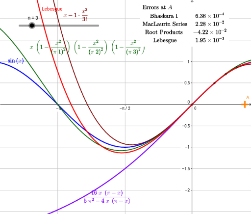
This example illustrates three Taylor series approximations of the sine function near zero. It covers core calculus concepts like Taylor expansion, polynomial approximation, and function graphing. Construction utilizes GeoGebra commands such as TaylorSeries, Point, ScientificText, Join, and If to generate polynomials and display values dynamically. Suitable for high school or college calculus students to visualize infinite series convergence.
GeoGebra Commands & Parameters
TaylorSeries(sin(x), 0, n) → TaylorCell(3, n + 1) → aPoint(xAxis) → AScientificText(errP, 3) → ePScientificText(errR, 3) → eRScientificText(errT, 3) → eTJoin({G1, {F2}}) → G2Join({G2, {F3}}) → G3Join({G3, {F4}}) → G4Join({G4, {F5}}) → G5Join({G5, {F6}}) → G6Join({G6, {F7}}) → G7Join({G7, {F8}}) → G8Join({G8, {F9}}) → G9Join({G9, {F10}}) → G10Join({G10, {F11}}) → G11Join({G11, {F12}}) → G12Join({G12, {F13}}) → G13Join({G13, {F14}}) → G14Join({G14, {F15}}) → G15Join({G15, {F16}}) → G16Join({G16, {F17}}) → G17If(n < 17, Cell[7, n + 1], Cell[7, 17]) → pntlistPolynomial(pntlist) → LebesgueScientificText(errL, 3) → eL
AI Drawing Prompt Reference
Plot the Taylor series approximations of the sine function near zero, including cubic, quintic, and septic polynomial approximations, and their respective errors. Start by drawing the sine function, then sequentially draw the cubic, quintic, and septic Taylor polynomial approximations, display the error for each polynomial, and connect these errors with curves.
The prompt above was compiled from the original drawing commands and is for reference only.