
Velocity Addition II: Geometric Demonstration of Relative Velocity
Loading the math board and drawing, please wait…
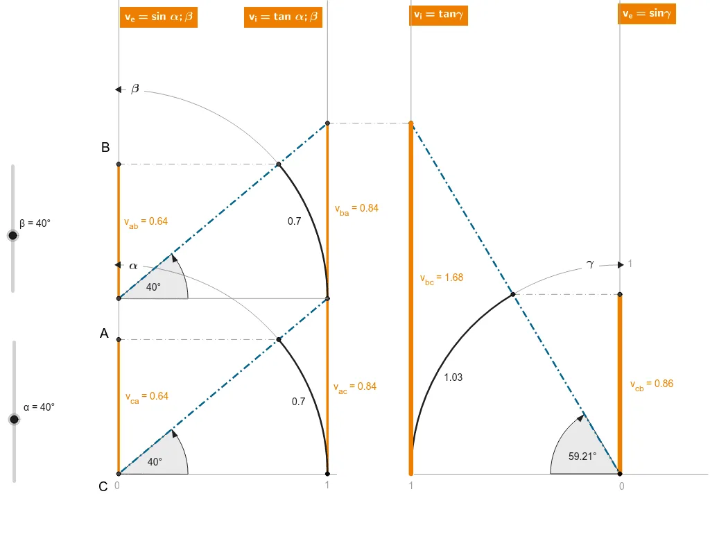
① This GeoGebra example dynamically illustrates the principle of velocity addition (relative velocity) in classical mechanics, showing how velocities from two moving reference frames combine vectorially. ② Core mathematical concepts include vector addition, velocity decomposition, relative motion, and trigonometric functions (cosine, secant) applied within a velocity triangle, with angles and segment lengths linked interactively. ③ Construction highlights: based on the summary, commands such as Point, Ray, OrthogonalLine, Rotate, Angle, Intersect, Segment, CircleArc, Line, Midpoint, and Circle are used to build a complete geometric model featuring velocity vectors, reference lines, circular arcs, and angle labels, likely controlled by sliders or dynamic points. ④ Suitable for high school physics or introductory university mechanics courses on relative motion and velocity composition, as well as mathematics classes demonstrating the geometric meaning of vector addition and trigonometric relationships.
GeoGebra Commands & Parameters
Point(yAxis) → BPoint(xAxis) → CPoint(yAxis) → ARay(A, B) → aRay(A, C) → bOrthogonalLine(C, b) → dRotate(C, α, A) → C'Ray(A, C') → eAngle(C, A, Rotate[C, α, A]) → α_1OrthogonalLine(C', b) → fOrthogonalLine(C', a) → gIntersect(g, a) → VeIntersect(f, b) → τSegment(A, Ve) → v_{ca}Segment(A, τ) → cosinusIntersect(e, d) → Vi2Segment(C, Vi2) → v_{ac}Segment(A, Vi2) → SecansIntersect(f, g) → DCircleArc(A, C, D) → ArcLine(Vi2, b) → hSegment(Ve, C') → iSegment(C', τ) → jPoint(Arc) → FMidpoint(D, A) → JCircle(J, A) → pRay(D, Vi2) → qPoint(d) → KSegment(K, C) → rPoint(q) → LSegment(Ve, D) → sSegment(D, τ) → tMidpoint(Vi2, D) → MPoint(q) → OSegment(Vi2, A) → secansRay(A, Vi2) → a_1Ray(A, Vi2) → kSegment(D, Vi2) → exsecMidpoint(D, A) → PCircleArc(A, C, B) → cIntersect(h, yAxis) → EPoint(Circle[E, 1]) → QSegment(E, Q) → lCircleArc(E, Vi2, Q) → c_1Rotate(Vi2, β, E) → Vi2'Angle(Vi2, E, Vi2') → γRay(E, Vi2') → mIntersect(m, r) → RSegment(E, R) → nSegment(Vi2, R) → v_{ba}CircleArc(E, Vi2, Vi2') → d_1Line(Vi2', h) → e_1Intersect(e_1, yAxis) → SSegment(S, Vi2') → f_1Segment(E, S) → v_{ab}Point(xAxis) → TLine(T, yAxis) → h_1Segment(E, Vi2) → i_1Point(h_1) → USegment(T, U) → j_1Line(R, xAxis) → k_1Intersect(k_1, j_1) → WSegment(R, W) → l_1Segment(T, W) → v_{bc}Point(Circle[T, 1]) → ZSegment(T, Z) → n_1Line(Z, j_1) → p_1Point(p_1) → A_1Segment(Z, A_1) → q_1Point(Circle[Z, 1]) → B_1CircleArc(Z, B_1, T) → r_1Segment(W, Z) → s_1Intersect(r_1, s_1) → C_1,CircleArc(Z, C_1, T) → t_1Line(C_1, xAxis) → a_2Intersect(a_2, q_1) → D_1Segment(Z, D_1) → v_{cb}Segment(D_1, C_1) → c_2Angle(T, Z, C_1) → δ
AI Drawing Prompt Reference
Draw a dynamic illustration showing the principle of velocity addition (relative velocity) in classical mechanics, combining velocities from two moving reference frames vectorially. The diagram should feature a velocity triangle with angles and segment lengths, interactive controls via sliders or dynamic points. Include velocity vectors, reference lines, circular arcs, and angle labels to demonstrate vector addition, velocity decomposition, relative motion, and trigonometric functions (cosine, secant).
The prompt above was compiled from the original drawing commands and is for reference only.