
Motion Symmetry: Preserving the Mass Centre
Loading the math board and drawing, please wait…
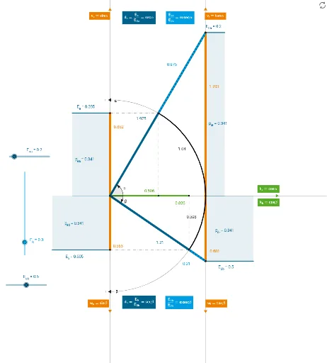
This GeoGebra example visually demonstrates the invariance of the mass center under motion symmetry. Using a combination of geometric construction commands—including Point, Segment, CircleArc, Intersect, Ray, OrthogonalLine, Angle, Line, and Polygon—the construction tracks how specific transformations preserve the mass center position. Core mathematical concepts include symmetry, center of mass, geometric transformations, and trigonometric relationships. The example is suitable for high school mathematics, physics, and geometry transformation units, supporting both conceptual understanding and dynamic exploration.
GeoGebra Commands & Parameters
Point(yAxis) → RPoint(yAxis) → ASegment(A, S) → iPoint(xAxis) → CPoint(yAxis) → BCircleArc(A, R, B) → cIntersect(c, i) → T,Ray(A, C) → bOrthogonalLine(C, b) → dCircleArc(A, C, T) → ArcPoint(d) → KAngle(C, A, Rotate[C, alfa, A]) → αOrthogonalLine(T, yAxis) → jOrthogonalLine(T, xAxis) → lIntersect(j, yAxis) → UIntersect(l, xAxis) → VSegment(A, V) → cosinusSegment(A, U) → sinusSegment(U, T) → sSegment(V, T) → tSegment(C, S) → tangensPoint(yAxis) → DPoint(yAxis) → LPoint(d) → MSegment(A, J) → mIntersect(c, m) → O,OrthogonalLine(O, yAxis) → nOrthogonalLine(O, xAxis) → pIntersect(p, xAxis) → PIntersect(n, yAxis) → QSegment(C, J) → qSegment(A, Q) → rSegment(A, P) → b_1Angle(J, A, V) → βSegment(P, O) → eSegment(O, Q) → fPoint(xAxis) → WCircleArc(A, O, C) → gSegment(T, S) → aSegment(J, O) → hSegment(V, Q) → kLine(C, k) → a_1Intersect(a_1, yAxis) → FLine(F, xAxis) → c_1Line(S, xAxis) → d_1Point(d_1) → GLine(G, yAxis) → e_1Intersect(e_1, c_1) → HSegment(G, H) → v_{ab}Segment(G, S) → g_1Segment(H, F) → h_1Segment(F, C) → i_1Polygon(A, B_1, N, U) → p_{ea}, a_2, b_2, E_{a}, uPolygon(C_1, Z, Q, A) → p_{eb}, c_2, E_{b}, q_1, a_3Polygon(C, S, D_1, D_2) → p_{ia}, c_3, E_{0a}, d_2, d_3Polygon(C, F_2, F_1, J) → p_{ib}, c_4, f_2, E_{0b}, j_1