
Varying Quantities of Red and Blue Paint on a Line
Loading the math board and drawing, please wait…
In collections
The variable-parts perspective across the curriculum
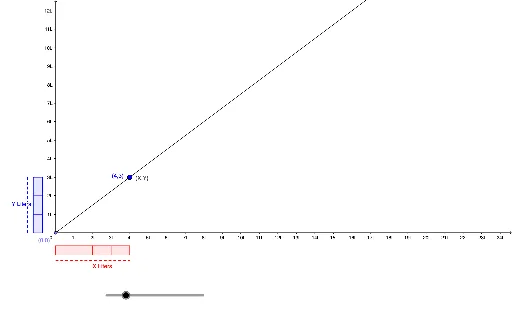
This GeoGebra example dynamically illustrates how varying quantities of red and blue paint relate along a straight line, using sliders or moving points to show proportional changes and total amounts. The core mathematical concepts include linear relationships, ratios, coordinate geometry, and geometric transformations such as scaling or translation via matrices. The construction employs commands like Point, Line, OrthogonalLine, Circle, Intersect, Polygon, Segment, and Ray to build base elements, with a slider (e.g., 'size') controlling variables, resulting in scatter plots or pyramid-like visual structures. It is suitable for middle and high school students learning linear functions, proportions, and transformations, as well as for teachers demonstrating dynamic mathematical modeling.
GeoGebra Commands & Parameters
Point(yAxis) → APoint(xAxis) → BLine(A, B) → aOrthogonalLine(A, a) → bCircle(A, 0.7) → cIntersect(c, a, 1) → CIntersect(c, b, 1) → DCircle(D, 0.5) → dCircle(C, 0.5) → eIntersect(e, a, 1) → EIntersect(d, b, 1) → FLine(D, a) → fLine(F, f) → gLine(C, b) → hLine(E, b) → iCircle(F, size) → kIntersect(k, g, 2) → GCircle(G, size) → pIntersect(p, g, 2) → HCircle(H, size) → qIntersect(q, g, 2) → ICircle(I, size) → rIntersect(r, g, 2) → JCircle(J, size) → sIntersect(s, g, 2) → KIntersect(a, i) → LCircle(E, size) → tIntersect(t, i, 2) → MCircle(M, size) → c_1Intersect(c_1, i, 2) → NCircle(N, size) → d_1Intersect(d_1, i, 2) → OOrthogonalLine(G, g) → jOrthogonalLine(H, g) → lOrthogonalLine(I, g) → mOrthogonalLine(J, g) → nOrthogonalLine(K, g) → a_1OrthogonalLine(M, i) → b_1OrthogonalLine(N, i) → e_1OrthogonalLine(O, i) → f_1Intersect(a_1, f_1) → PIntersect(a_1, f_1) → QIntersect(h, f_1) → RIntersect(h, e_1) → SIntersect(h, b_1) → TIntersect(f, j) → UIntersect(f, l) → VIntersect(f, m) → WIntersect(f, n) → ZIntersect(f, a_1) → A_1Polygon(D, F, G, U) → poly1, d_2, f_2, g_1, uPolygon(U, G, H, V) → poly2, u_1, g_2, h_1, vPolygon(H, I, W, V) → poly3, h_2, i_1, w, v_1Polygon(E, C, T, M) → poly6, e_2, c_2, t_1, m_1Polygon(T, S, N, M) → poly7, t_2, s_1, n_1, m_2Polygon(S, R, O, N) → poly8, s_2, r_1, o, n_2Circle(F, 0.3) → p_1Circle(K, 0.3) → q_1Circle(O, 0.3) → k_2Circle(E, 0.3) → p_2Intersect(k_2, f_1, 2) → B_1Intersect(p_2, a, 1) → C_1Intersect(p_1, b, 1) → D_1Intersect(q_1, a_1, 1) → E_1Intersect(x = 5, y = 3) → F_1Circle(O, size) → k_1Intersect(k_1, i, 2) → G_1OrthogonalLine(G_1, i) → j_1Intersect(h, j_1) → H_1Polygon(O, R, H_1, G_1) → poly4, o_1, r_2, h_3, g_3Circle(G_1, 0.3) → q_2Intersect(q_2, j_1, 2) → I_1Circle(I, 0.3) → c_3Intersect(c_3, m, 1) → J_1Segment(D_1, J_1) → l_1Segment(I_1, C_1) → a_2Intersect(m, j_1) → K_1Intersect(x = 3, y = 4) → L_1Ray(A, L_1) → b_2Circle(J, 0.3) → d_3Intersect(d_3, n, 1) → M_1Segment(D_1, M_1) → i_2Segment(C_1, B_1) → j_2Polygon(W, I, J, Z) → poly5, w_1, i_3, j_3, z_1Intersect(n, f_1) → N_1Ray(A, N_1) → l_2
AI Drawing Prompt Reference
Draw a straight line and mark two points on it. Create two circles with different radii centered at these points, and find their intersections with the line. Construct additional circles and lines using these intersection points to form a complex geometric pattern. Use a slider to control the size of some circles, showing dynamic changes. The overall design should illustrate linear relationships and proportional changes, suitable for educational purposes.
The prompt above was compiled from the original drawing commands and is for reference only.