
Uniform Acceleration Motion Demo
Loading the math board and drawing, please wait…
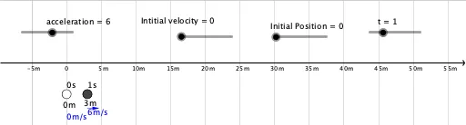
This example demonstrates the relationship between displacement, velocity, and time in uniform acceleration motion. It involves core math concepts like function graphs, linear functions, quadratic functions, derivatives, and limits. The construction uses the Sequence command to generate trajectory points, slider animations to show velocity vectors and changes in position/velocity over time, and labels key data. Suitable for high school physics and math education to understand the mathematical expressions and geometric meanings of acceleration, velocity, and displacement.
GeoGebra Commands & Parameters
Sequence((((0.5 * acceleration) * i^(2)) + (initialVelocity * i) + initialPosition, 0 - Yscale / 2), i, 0, t) → pointsSequence(Text[(acceleration * i) + initialVelocity + positionUnit + "/" + timeUnit, (((0.5 * acceleration) * i^(2)) + (initialVelocity * i) + initialPosition + Yscale / 100, 0 - (Yscale / 2.7 * (1 + (0.1 * (-1)^(i)))) - Yscale / 2)], i, 0, t) → velocityLabelsSequence(Vector[(((0.5 * acceleration) * i^(2)) + (initialVelocity * i) + initialPosition, (((-Yscale)) / 4 * (1 + (0.1 * (-1)^(i)))) - Yscale / 2), (((0.5 * acceleration) * i^(2)) + (initialVelocity * i) + initialPosition + (((acceleration * i) + initialVelocity) * Xscale / 200), (((-Yscale)) / 4 * (1 + (0.1 * (-1)^(i)))) - Yscale / 2)], i, 0, t) → velocityVectorsSequence(Text[i + timeUnit, (((0.5 * acceleration) * i^(2)) + (initialVelocity * i) + initialPosition, 0 + Yscale / 10 - Yscale / 2)], i, 0, t) → timeLabelsSequence(Text[((0.5 * acceleration) * i^(2)) + (initialVelocity * i) + initialPosition + positionUnit, (((0.5 * acceleration) * i^(2)) + (initialVelocity * i) + initialPosition, 0 - ((Yscale * 0.2) * (1 + (0.1 * (-1)^(i))))) - Yscale / 2], i, 0, t) → PositionValueLabels
AI Drawing Prompt Reference
Illustrate the relationship between displacement, velocity, and time in uniform acceleration motion by plotting a parabolic trajectory, showing velocity vectors, and labeling key data and time points with animation to demonstrate changes in velocity and position over time.
The prompt above was compiled from the original drawing commands and is for reference only.