
UCSS Math I 4.3.3 Example 2: Correlation between Study Time and Test Performance
Loading the math board and drawing, please wait…
In collections
UCSS Secondary Math I Unit 4 Lesson 3
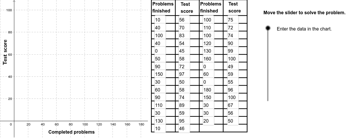
This example demonstrates how to analyze the correlation between study time and test performance using a scatter plot and a fitted line. The core mathematical concepts include Pearson's correlation coefficient (PMCC), linear regression (least squares fitting), and data visualization. The construction uses GeoGebra commands such as FitLineY to generate the best-fit line, PMCC to compute the correlation coefficient, Textfield for data input, Polygon and Sequence for constructing data points or auxiliary shapes, and Segment and RotateText for annotations and text rotation. It is suitable for high school or introductory college statistics courses to illustrate real-world applications of correlation and regression analysis.
GeoGebra Commands & Parameters
FitLineY(PointList1) → LineFitPMCC(PointList1) → CorCoeffTextfield(A2) → InA2Textfield(A3) → InA3Textfield(A4) → InA4Textfield(A5) → InA5Textfield(A6) → InA6Textfield(A7) → InA7Textfield(A8) → InA8Textfield(A9) → InA9Textfield(A10) → InA10Textfield(A11) → InA11Textfield(A12) → InA12Textfield(A13) → InA13Textfield(A14) → InA14Textfield(A15) → InA15Textfield(A16) → InA16Textfield(A17) → InA17Textfield(A18) → InA18Textfield(A19) → InA19Textfield(A20) → InA20Textfield(A21) → InA21Textfield(B2) → InB2Textfield(B3) → InB3Textfield(B4) → InB4Textfield(B5) → InB5Textfield(B6) → InB6Textfield(B7) → InB7Textfield(B8) → InB8Textfield(B9) → InB9Textfield(B10) → InB10Textfield(B11) → InB11Textfield(B12) → InB12Textfield(B13) → InB13Textfield(B14) → InB14Textfield(B15) → InB15Textfield(B16) → InB16Textfield(B17) → InB17Textfield(B18) → InB18Textfield(B19) → InB19Textfield(B20) → InB20Textfield(B21) → InB21Polygon((190, y(Corner[1])), Corner[2], Corner[3], (190, y(Corner[4]))) → poly1, a, b, c, dTextfield(A22) → InA22Textfield(A23) → InA23Textfield(A24) → InA24Textfield(A25) → InA25Textfield(A26) → InA26Textfield(B22) → InB22Textfield(B23) → InB23Textfield(B24) → InB24Textfield(B25) → InB25Textfield(B26) → InB26Textfield(A27) → InA27Textfield(A28) → InA28Textfield(A29) → InA29Textfield(A30) → InA30Textfield(B27) → InB27Textfield(B28) → InB28Textfield(B29) → InB29Textfield(B30) → InB30Sequence(Segment[(195, (-10) + (7 * i)), (331, (-10) + (7 * i))], i, 0, 15) → Linesh1Sequence(Segment[(195 + (34 * i), (-10)), (195 + (34 * i), 109)], i, 0, 4) → Linesv1Segment((195, 109), (331, 109)) → top1RotateText("Test score", 90*°) → SideLegend
AI Drawing Prompt Reference
Create a scatter plot showing the relationship between study time and test scores, with a fitted line to illustrate the trend. Include the calculated correlation coefficient and text fields for data input. The plot should feature multiple data points, a best-fit line, labeled correlation coefficient, and input fields.
The prompt above was compiled from the original drawing commands and is for reference only.