
UCSS Math I 4.2.3 Example 1: Plant Growth Height Data and Linear Function Modeli
Loading the math board and drawing, please wait…
In collections
UCSS Secondary Math I Unit 4 Lesson 2
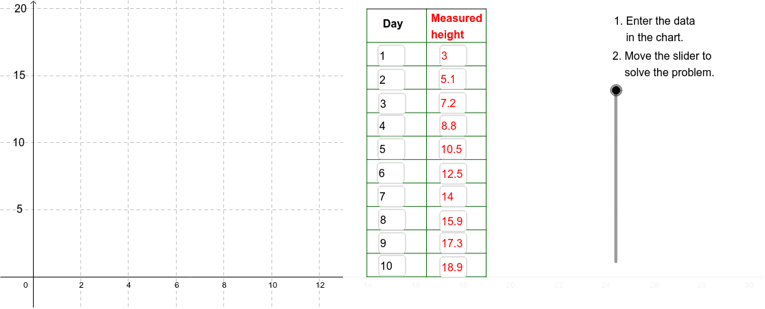
This example demonstrates how to plot daily plant height measurements as a scatter of points in a coordinate system and then model the growth trend using a linear function. The core mathematical concepts include linear functions, sequences of data points, the geometric meaning of slope and intercept, and using function graphs for prediction. Construction highlights: the GeoGebra commands Sequence, Textfield, Segment, and Polygon are used to generate the ordered data points, input values, connect adjacent points to visualize growth, and construct auxiliary polygons (e.g., rectangles representing daily increments). This resource is suitable for middle and high school students learning linear functions and data modeling, and can be used in math lab activities to guide students from real-world data to abstract function relationships.
GeoGebra Commands & Parameters
Sequence(Segment[(11.5, (5 * i)), (12.5, (5 * i))], i, 1, 4) → TickListTextfield(A2) → InA2Textfield(A3) → InA3Textfield(A4) → InA4Textfield(A5) → InA5Textfield(A6) → InA6Textfield(A7) → InA7Textfield(A8) → InA8Textfield(A9) → InA9Textfield(A10) → InA10Textfield(A11) → InA11Textfield(B2) → InB2Textfield(B3) → InB3Textfield(B4) → InB4Textfield(B5) → InB5Textfield(B6) → InB6Textfield(B7) → InB7Textfield(B8) → InB8Textfield(B9) → InB9Textfield(B10) → InB10Textfield(B11) → InB11Sequence(Segment[(14, 0 + (1.75 * i)), (19, 0 + (1.75 * i))], i, 0, 10) → CrossList1Sequence(Segment[(19, 0 + (1.75 * i)), (21.5, 0 + (1.75 * i))], i, 0, 10) → CrossList2Sequence(Segment[(21.5, 0 + (1.75 * i)), (24, 0 + (1.75 * i))], i, 0, 10) → CrossList3Sequence(Segment[(14 + (2.5 * i), 0), (14 + (2.5 * i), 20)], i, 0, 2) → SideList1Segment((14, 20), (19, 20)) → Top1Segment((19, 20), (21.5, 20)) → Top2Segment((21.5, 20), (24, 20)) → Top3Segment((21.5, 0), (21.5, 20)) → Side2Segment((24, 0), (24, 20)) → Side3Polygon((13, y(Corner[1])), Corner[2], Corner[3], (13, y(Corner[4]))) → poly1, b, c, d, eSegment((0, 10), (13, 10)) → ResidualAxis
AI Drawing Prompt Reference
Draw a coordinate plane with the x-axis representing days and the y-axis representing plant height. Plot daily height measurements as scattered points in order, then connect adjacent points with line segments to show the growth trend. Below the data points, place several input boxes for entering values. On the right side of the graph, construct a grid framework made of horizontal and vertical lines, forming multiple rectangular areas to represent daily increments. Near the bottom of the coordinate plane, draw a horizontal reference line for the residual axis. The overall layout should clearly show the data points, connecting lines, input areas, and auxiliary grid to visualize the linear growth relationship.
The prompt above was compiled from the original drawing commands and is for reference only.