
Two Distributions - Mode, Median, Expected Value
Loading the math board and drawing, please wait…
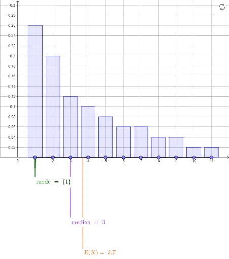
This example demonstrates the calculation and visualization of mode, median, and expected value for two different distributions. Key math concepts include probability & statistics on distributions, mode, median, expected value, and coordinate geometry for data representation. Construction highlights GeoGebra commands like Segment, Point, mean, Median, If, Length, Sequence, and BarChart. Suitable for high school and above students learning probability statistics and data analysis.
GeoGebra Commands & Parameters
Segment((1, 0), (11, 0)) → thexaxisPoint(thexaxis) → A12Point(thexaxis) → A13Point(thexaxis) → A14Point(thexaxis) → A15Point(thexaxis) → A16Point(thexaxis) → A17Point(thexaxis) → A18Point(thexaxis) → A19Point(thexaxis) → A20Point(thexaxis) → A21Point(thexaxis) → A22Point(thexaxis) → A23Point(thexaxis) → A24Point(thexaxis) → A25Point(thexaxis) → A26Point(thexaxis) → A27Point(thexaxis) → A28Point(thexaxis) → A29Point(thexaxis) → A30Point(thexaxis) → A31Point(thexaxis) → A32Point(thexaxis) → A33Point(thexaxis) → A34Point(thexaxis) → A35Point(thexaxis) → A36Point(thexaxis) → A37Point(thexaxis) → A38Point(thexaxis) → A39Point(thexaxis) → A40Point(thexaxis) → A41Point(thexaxis) → A42Point(thexaxis) → A43Point(thexaxis) → A44Point(thexaxis) → A45Point(thexaxis) → A46Point(thexaxis) → A47Point(thexaxis) → A48Point(thexaxis) → A49Point(thexaxis) → A50Point(thexaxis) → B13Point(thexaxis) → B14Point(thexaxis) → B15Point(thexaxis) → B16Point(thexaxis) → B17Point(thexaxis) → B18Point(thexaxis) → B19Point(thexaxis) → B20Point(thexaxis) → B21Point(thexaxis) → B22Point(thexaxis) → B23Point(thexaxis) → B24Point(thexaxis) → B25Point(thexaxis) → B26Point(thexaxis) → B27Point(thexaxis) → B28Point(thexaxis) → B29Point(thexaxis) → B30Point(thexaxis) → B31Point(thexaxis) → B32Point(thexaxis) → B33Point(thexaxis) → B34Point(thexaxis) → B35Point(thexaxis) → B36Point(thexaxis) → B37Point(thexaxis) → B38Point(thexaxis) → B39Point(thexaxis) → B40Point(thexaxis) → B41Point(thexaxis) → B42Point(thexaxis) → B43Point(thexaxis) → B44Point(thexaxis) → B45Point(thexaxis) → B46Point(thexaxis) → B47Point(thexaxis) → B48Point(thexaxis) → B49Point(thexaxis) → B50mean(thexs1) → mean1mean(thexs2) → mean2Median(thexs1) → median1Median(thexs2) → median2If(Length[Mode[thexs1]] ≟ 0, Sequence[10], Mode[thexs1]) → mode1If(Length[Mode[thexs2]] ≟ 0, Sequence[10], Mode[thexs2]) → mode2Length(mode1) → nummode1Length(mode2) → nummode2Segment((median1, (mediandepth * ymin)), (median1, 0)) → meadianpos1Segment((mean1, (meandepth * ymin)), (mean1, 0)) → meanpos1Segment((median2, (mediandepth * ymin)), (median2, 0)) → medianpos2Segment((mean2, (meandepth * ymin)), (mean2, 0)) → meanpos2Sequence(Segment[(mode1(i), ((1 / 2 * modedepth) * ymin)), (mode1(i), 0)], i, 1, nummode1) → modepos1Sequence(Segment[(mode2(i), ((1 / 2 * modedepth) * ymin)), (mode2(i), 0)], i, 1, nummode2) → modepos2Segment((Min[mode1], ((1 / 2 * modedepth) * ymin)), (Max[mode1], ((1 / 2 * modedepth) * ymin))) → modebar1Segment((Min[mode2], ((1 / 2 * modedepth) * ymin)), (Max[mode2], ((1 / 2 * modedepth) * ymin))) → modebar2Segment(((Min[mode1] + Max[mode1]) / 2, (modedepth * ymin)), ((Min[mode1] + Max[mode1]) / 2, ((1 / 2 * modedepth) * ymin))) → modelabel1Segment(((Min[mode2] + Max[mode2]) / 2, (modedepth * ymin)), ((Min[mode2] + Max[mode2]) / 2, ((1 / 2 * modedepth) * ymin))) → modelabel2Point(thexaxis) → B12BarChart(Sequence[11], freq1, 0.8) → dist1BarChart(Sequence[11], freq2, 0.8) → dist2Point(thexaxis) → A11Point(thexaxis) → B11Point(thexaxis) → A1Point(thexaxis) → A2Point(thexaxis) → A3Point(thexaxis) → A4Point(thexaxis) → A5Point(thexaxis) → A6Point(thexaxis) → A7Point(thexaxis) → A8Point(thexaxis) → A9Point(thexaxis) → A10Point(thexaxis) → B1Point(thexaxis) → B2Point(thexaxis) → B3Point(thexaxis) → B4Point(thexaxis) → B5Point(thexaxis) → B6Point(thexaxis) → B7Point(thexaxis) → B8Point(thexaxis) → B9Point(thexaxis) → B10
AI Drawing Prompt Reference
Draw two distribution curves representing two different distributions. Mark the mode, median, and expected value on the x-axis for each distribution. The mode is where the peak of the curve is, the median is a vertical line that splits the curve in half, and the expected value is the center of the area under the curve.
The prompt above was compiled from the original drawing commands and is for reference only.