Binomial Distribution with 1000 Trials - Dynamic Bar Chart

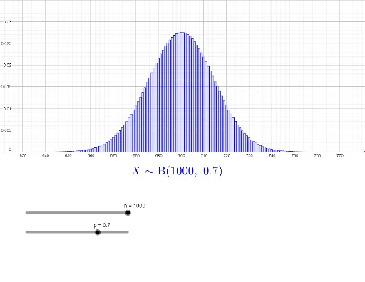
① This GeoGebra example demonstrates the probability distribution of a binomial experiment with 1000 trials using a dynamic bar chart, showing how probabilities vary across different numbers of successes. ② The core mathematical concept is the binomial distribution, involving parameters n (number of trials) and p (probability of success), along with the probability mass function and its visualization. ③ Construction details: The Sequence command generates the sequence of trial counts, BarChart creates the bar chart, and objects such as n, p, thexs (success counts), thefreqs (frequencies), thedist (distribution values), ymax/ymin/xmax/xmin (coordinate ranges), and text1 (text label) are defined. Sliders allow real-time adjustment of parameters to update the graph. ④ Suitable for high school and university probability and statistics courses, this tool helps students understand how the binomial distribution shape changes with n and p, and serves as an interactive demonstration for teachers or self-study.