
Truncated Icosidodecahedron: Relationship Between Average Distance and Truncatio
Loading the math board and drawing, please wait…
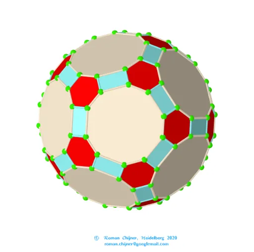
This example demonstrates a truncated icosidodecahedron and explores the relationship between the average distance between vertices and the truncation parameter. By adjusting the truncation parameter, extreme distributions of vertices can be observed. Commands used include Join, Unique, Length, Text, Sum, Sphere, Ray, Zip, UnicodeToLetter, and TableText. Suitable for high school mathematics education and research.
GeoGebra Commands & Parameters
Join(Zip[lP0(x(a)) + ((lP0(y(a)) - lP0(x(a))) * {t, 1 - t}), a, segN]) → lVVUnique(lVV) → lP'Length(lP') → nLength(lVV(1)) → R2Text("" + p3) → txt_pSum(Flatten[Sequence[Append[Sequence[Element[txt_p, i], i, m1(k), m2(k)], " "], k, 1, 5]]) → txtUm1Sphere(O, R1) → sp1Sphere(O, R2) → sp2Ray(B, AA) → hText(text12, C, false, true) → text8Zip(Segment[lP0(x(a)), lP0(y(a))], a, segN1) → seg1Zip(Segment[lP0(x(a)), lP0(y(a))], a, segN2) → seg2Zip(Polygon[a], a, v_poly06) → poly06Zip(Polygon[a], a, v_poly04) → poly04Zip(Polygon[a], a, v_poly10) → poly10UnicodeToLetter(34) → u34Zip(Segment[lVV(x(a)), lVV(y(a))], a, segNΔ4) → segΔ4Zip(Segment[lVV(x(a)), lVV(y(a))], a, segNΔ6) → segΔ6Zip(Segment[lVV(x(a)), lVV(y(a))], a, segNΔ10) → segΔ10TableText(Append["\;\;\; \fgcolor{#0087BD}{4-gons}", segΔ4], Append["\;\;\; \fgcolor{red}{6-gons}", segΔ6], Append["\;\;\; \fgcolor{#79443B}{10-gons}", segΔ10], "v") → text3a
AI Drawing Prompt Reference
Draw a truncated icosidodecahedron and explore the change in average vertex distance by adjusting the truncation parameter. First, create the edges of the truncated icosidodecahedron, then calculate all vertices, followed by the number of vertices and radii under the truncation parameter, and finally show the distribution of polygons for different truncation parameters.
The prompt above was compiled from the original drawing commands and is for reference only.