
Trigonometric Functions & Integral Integration
Loading the math board and drawing, please wait…
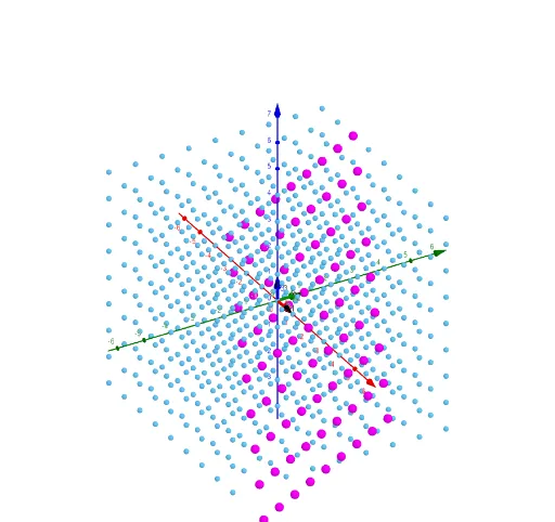
This example demonstrates the integration of trigonometric functions, scalene triangles, definite integrals, and hyperbolas. It uses dynamic constructions to illustrate vector matrix transformations and the positional relationships of orthogonal planes and points. Commands like ApplyMatrix, OrthogonalPlane, PointIn, and Sequence are applied, involving operations on vectors e1, e2, e3, t1, t2, t3, and the dynamic generation of points P, B, B'. Suitable for high school and above students to understand the combination of calculus and linear algebra.
GeoGebra Commands & Parameters
ApplyMatrix(M, e_{1}) → t_{1}ApplyMatrix(M, e_{2}) → t_{2}ApplyMatrix(M, e_{3}) → t_{3}OrthogonalPlane((0, 0, 0), Vector[t_{1} ⊗ t_{2}]) → dOrthogonalPlane((0, 0, 0), Vector[t_{1} ⊗ t_{3}]) → eOrthogonalPlane((0, 0, 0), Vector[t_{2} ⊗ t_{3}]) → fOrthogonalPlane(P, Vector[u ⊗ v]) → aPointIn(a) → BApplyMatrix(M, B) → B'Sequence(Sequence[(n - (2 * w) + t, w, t), w, -4, 4, 1], t, -4, 4, 1) → m1ApplyMatrix(M, m1) → m1'Sequence(Sequence[Sequence[(x_{1}, x_{2}, x_{3}), x_{1}, -4, 4, 1], x_{2}, -4, 4, 1], x_{3}, -4, 4, 1) → l1ApplyMatrix(M, l1) → l1'
AI Drawing Prompt Reference
Illustrate the integration of trigonometric functions and vector matrix transformations, including orthogonal planes and points, demonstrating vector matrix transformations and positional relationships of orthogonal planes dynamically, generating points B and B', and drawing a grid generated by trigonometric functions and its transformed version to show the combination of calculus and linear algebra.
The prompt above was compiled from the original drawing commands and is for reference only.