
Second Pendulum Demo
Loading the math board and drawing, please wait…
In collections
El dominio del Tiempo (cinemática intuitiva)
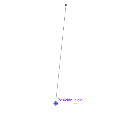
This example demonstrates the 2D motion trajectory and vector changes of a second pendulum. It involves core mathematical concepts like 2D vectors, geometric construction, limits, derivatives, and parametric equations. Construction highlights include using GeoGebra commands such as Circle, Rotate, and UnitOrthogonalVector to draw trajectories and dynamic graphics. Suitable for high school students and math enthusiasts exploring the intersection of physics and mathematics.
GeoGebra Commands & Parameters
Circle(O, l) → cRotate(O + (0, (-l)), -8°, O) → ARotate(O + (0, (-l)), 8°, O) → A'CircleArc(O, A, A') → arcPoint(arc) → PPoint(c) → MSegment(O, M) → rUnitOrthogonalVector(r) → nIf(Length[reg] ≟ 1, {reg(1)}, Sequence[reg(k) - reg(k + 1), k, 1, Length[reg] - 1]) → regDifmean(regDif) → TAngle(P, O, (x(O), -100)) → ampSum(Sequence[((((2 * k))! / ((2^((2 * k)) * (k!)^(2))))^(2) * (sin(amp / 2))^((2 * k))), k, 0, 83]) → sumSegment(O, P) → rPLine(M, gt) → i
AI Drawing Prompt Reference
Draw a second pendulum physical model, including a curved arc, a fixed point, a moving point, a radius, a unit orthogonal vector, a difference sequence, an average, an amplitude, and a sum. The curved arc is composed of two circular arcs with equal radii, centered at the fixed point above and below. The moving point is located on the curved arc, and the radius points to the fixed point. The unit orthogonal vector points to the radius. The difference sequence is composed of the differences between two consecutive arc lengths, and the average is the average of the difference sequence. The amplitude is the angle between the moving point and the fixed point. The sum is composed of multiple terms, each in the form of (2k)! / (2^(2k) * (k!)^2) * (sin(angle/2))^(2k).
The prompt above was compiled from the original drawing commands and is for reference only.