
Trigonometric Equations Self-Test
Loading the math board and drawing, please wait…
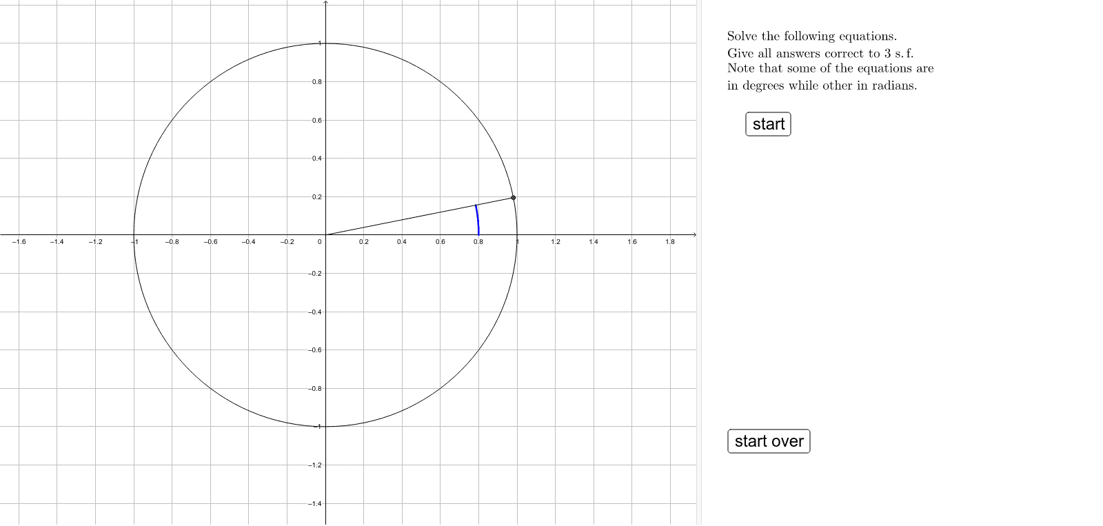
This example demonstrates the solving process of trigonometric equations through visual means, aiding in the understanding of the solutions. The core mathematical concepts involved include trigonometric functions, equation solving, and geometric representation. It is constructed using GeoGebra commands such as Element, Circle, Segment, Arc, If, Textfield, Polygon, Length, and objects like ans2, ans1, prnr, problem, sol2, sol1, c, s, d, P, Pc, Ps, pcos, psin, segmcos, segmsin, radP, radPc, radPs, e, arcPabove, f, arcPsabove, arcPcbelow, angleP, anglePc, anglePs, anglePdeg, anglePcdeg, anglePsdeg, textRad, started, textDeg, textRD, text1, eqn, text2, RD, text3, text4. Suitable for high school students and teachers.
GeoGebra Commands & Parameters
Element(Element[problem, prnr], 4) → sol2Element(Element[problem, prnr], 3) → sol1Circle((0, 0), 1) → dSegment(P, Pc) → segmcosSegment(P, Ps) → segmsinSegment((0, 0), P) → radPSegment((0, 0), Pc) → radPcSegment((0, 0), Ps) → radPsCircle((0, 0), 0.8) → eArc(e, (0, 0), P) → arcPaboveCircle((0, 0), 0.7) → fArc(f, (0, 0), Ps) → arcPsaboveArc(f, (0, 0), Pc) → arcPcbelowIf(s ≥ 0, acos(c), (-acos(c))) → anglePIf(s < 0, acos(c), (-acos(c))) → anglePcIf(s ≥ 0, acos((-c)), (-acos((-c)))) → anglePsElement(Element[problem, prnr], 1) → eqnElement(textRD, Element[Element[problem, prnr], 2] + 1) → RDTextfield(ans1) → InputBox1Textfield(ans2) → InputBox2Arc(e, (1, 0), P) → arcPbelowArc(f, (1, 0), Ps) → arcPsbelowArc(f, (1, 0), Pc) → arcPcabovePolygon(Corner[1], Corner[2], Corner[3], Corner[4]) → poly1, a, b, g, hLength(problem) → length