
Polynomial Inequalities: Self-Test
Loading the math board and drawing, please wait…
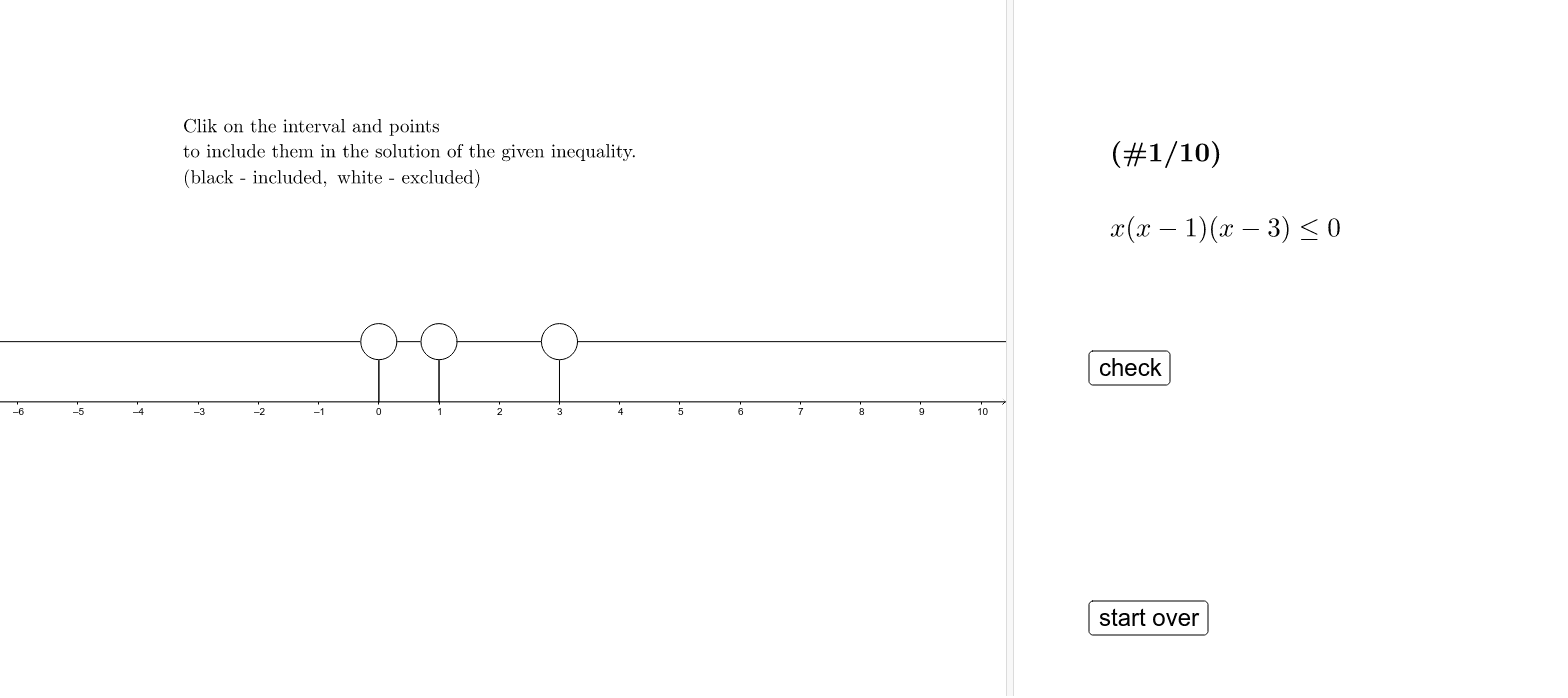
This example demonstrates the graphical representation of polynomial inequalities. Key mathematical concepts include polynomial functions, inequalities, and their solution sets. By constructing the roots of the polynomial function and the regions of the inequality solutions, students can deepen their understanding of polynomial inequalities. GeoGebra commands such as Element, Polygon, Circle, and Length are used. Suitable for high school mathematics education and learning.
GeoGebra Commands & Parameters
Element(Element[problem, prnr], 5) → codePolygon(Corner[1], Corner[2], Corner[3], Corner[4]) → poly1, a, b, c, dElement(Element[problem, prnr], 1) → intextElement(Element[problem, prnr], 2) → x1Element(Element[problem, prnr], 3) → x2Element(Element[problem, prnr], 4) → x3Polygon(Bx0, Bx1, Tx1, Tx0) → int1, bx0, bx1, tx1, tx0Polygon(Bx1, Bx2, Tx2, Tx1) → int2, bx1_1, bx2, tx2, tx1_1Polygon(Bx2, Bx3, Tx3, Tx2) → int3, bx2_1, bx3, tx3, tx2_1Polygon(Bx3, Bx4, Tx4, Tx3) → int4, bx3_1, bx4, tx4, tx3_1Circle(Tx1, 0.3) → eCircle(Tx2, 0.3) → fCircle(Tx3, 0.3) → gLength(problem) → length
AI Drawing Prompt Reference
Draw a graph of a polynomial inequality, including the roots x1, x2, x3 of the polynomial function, and the solution sets regions int1, int2, int3, int4. First, plot points x1, x2, x3 on the x-axis, then construct four regions for the solution sets based on these points, with each region defined by four points. Next, draw circles with radius 0.3 at the boundaries of each solution set region. Finally, connect the centers of these circles with lines to form a curve.
The prompt above was compiled from the original drawing commands and is for reference only.