
Temperature Variation Over Time in Physics
Loading the math board and drawing, please wait…
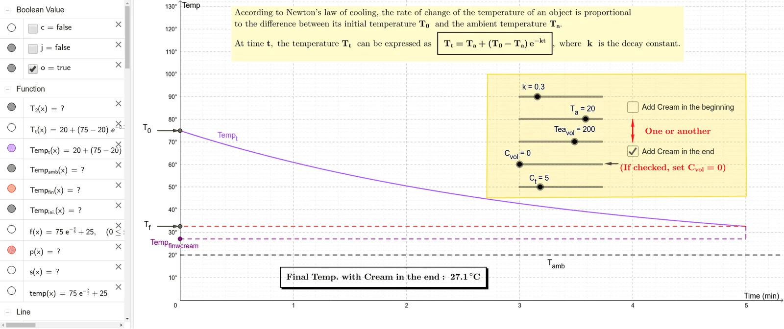
This example graphically solves a cooling problem in physics. Key mathematical concepts include functions, exponential functions, and differential equations. GeoGebra commands such as Segment, Vector, and Polygon are used in the construction. Suitable for high school physics and math courses, aiding students in understanding temperature changes over time.
GeoGebra Commands & Parameters
Segment((5, Temp_t(5)), C) → iVector(D, B) → T_0Vector(E, A) → T_fVector(F, G) → uVector(G, F) → vVector(H, I) → wPolygon(J, K, L, M) → c1, j_1, k_1, l, mSegment(Temp_{finwcream}, C) → nSegment((5, Temp_t(5)), A) → tSegment((0, T_a), (6, T_a)) → T_{amb}
AI Drawing Prompt Reference
Draw a graph showing temperature variation over time in a physics cooling process. First, draw vectors representing the initial temperature T₀ and final temperature T_f. Then, draw the function curve showing temperature change over time. Next, draw a horizontal line for the ambient temperature T_amb and vectors indicating the rate of temperature change. Finally, use a polygon to represent the area of temperature change.
The prompt above was compiled from the original drawing commands and is for reference only.