
Taylor Approximants of a Cubic Function
Loading the math board and drawing, please wait…
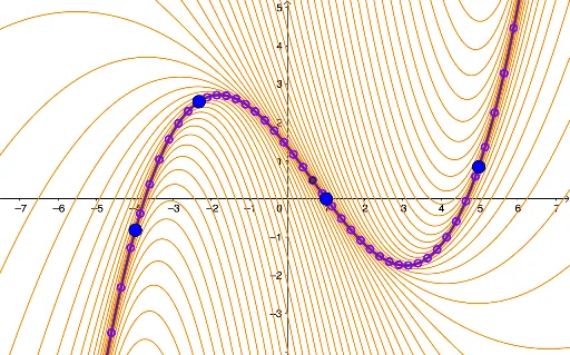
This example demonstrates the Taylor approximants of a cubic function. Key mathematical concepts include Taylor polynomials, polynomial functions, and derivatives. The construction uses the FitPoly command to build the polynomial approximations, and the TurningPoint and Sequence commands to illustrate key points in the approximation process. Suitable for teaching function approximation in calculus courses.
GeoGebra Commands & Parameters
FitPoly({A, B, C, D}, 3) → fTurningPoint(f) → ESequence((w + x(E), f(w + x(E))), w, -10, 10, 0.25) → l3Sequence(TaylorSeries[f, x(Element[l3, w]), 2], w, 1, Length[l3]) → l2
AI Drawing Prompt Reference
Draw a graph of Taylor approximations of a cubic function. Show a cubic polynomial function and its Taylor polynomial approximations. The graph includes the function curve, the Taylor polynomial curve, and key points like turning points. The construction order is to first draw the function curve, then add the Taylor polynomial, and finally mark the turning points to help understand the approximation process.
The prompt above was compiled from the original drawing commands and is for reference only.