
Surface with Square Cross Sections
Loading the math board and drawing, please wait…
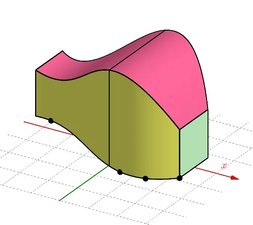
This example demonstrates how to build a 3D surface whose cross-sections are squares at different positions. By moving the slicing parameter, you can see how a square polygonal cross-section evolves along the surface, giving an intuitive visualization of how geometry changes under a varying cut. The key mathematics includes solid geometry (a parametric/constructed surface), Cartesian curve modeling, polygon construction (closed boundaries forming a square), and ideas linked to integral calculus (using constructed relations to study how section geometry accumulates or changes along a direction). Construction highlights from the GeoGebra command set include: CurveCartesian to create the guiding curves, Segment to define edges, Polygon to form the square cross-section from its vertices, Surface to generate the resulting 3D object, and PointIn/Vertex to manage key points on the section and surface. FitPoly supports fitting the profile/shape, Min/Max controls parameter ranges or extremal constraints, and Slider/SlideMe provides interactive control of the cut position so the square sections update dynamically. Suitable for advanced high-school and undergraduate learners in calculus and solid/analytic geometry, especially for classroom demos and exploratory modeling.
GeoGebra Commands & Parameters
PointIn(f) → APointIn(f) → BPointIn(f) → CPointIn(f) → DPointIn(f) → GPointIn(f) → HPointIn(f) → IPointIn(f) → JFitPoly({M, L, E, K}) → gFitPoly({P, N, O, F}) → hMin({x(M), x(L), x(E), x(K), x(P), x(N), x(O), x(F)}) → aMax({x(M), x(L), x(E), x(K), x(P), x(N), x(O), x(F)}) → bPolygon(Q, R, S, T) → q1, q_1, r, s_1, tSegment(Q, R) → iSegment(R, S) → jSegment(S, T) → kSegment(T, Q) → lCurveCartesian(t, q(t), abs(p(t) - q(t)), t, a, b) → cCurveCartesian(t, p(t), abs(p(t) - q(t)), t, a, b) → dSurface(u, p(u), (abs(p(u) - q(u)) * v), u, a, b, v, 0, 1) → eSurface(u, q(u), (abs(p(u) - q(u)) * v), u, a, b, v, 0, 1) → mSurface(u, q(u) + (abs(p(u) - q(u)) * v), abs(p(u) - q(u)), u, a, b, v, 0, 1) → nPolygon((a, p(a), 0), (a, p(a), abs(p(a) - q(a))), (a, q(a), abs(p(a) - q(a))), (a, q(a), 0)) → q2, f_1, g_1, h_1, i_1Vertex(q2, 1) → UVertex(q2, 2) → VVertex(q2, 3) → WVertex(q2, 4) → ZSegment(Z, U) → j_1Segment(U, V) → k_1Segment(V, W) → l_1Segment(W, Z) → m_1Polygon((b, p(b), 0), (b, p(b), abs(p(b) - q(b))), (b, q(b), abs(p(b) - q(b))), (b, q(b), 0)) → q3, n_1, p_1, r_1, t_1Vertex(q3, 1) → A_1Vertex(q3, 2) → B_1Vertex(q3, 3) → C_1Vertex(q3, 4) → D_1Segment(A_1, B_1) → a_1Segment(B_1, C_1) → b_1Segment(C_1, D_1) → c_1Segment(D_1, A_1) → d_1
AI Drawing Prompt Reference
Describe a 3D surface with square cross-sections at different heights. The squares move as height changes, forming a continuous surface. The surface is defined by two parameters: height and vertical direction. The square cross-section is formed by four points that move along the surface. Adjusting the height parameter allows observation of how the square changes. This illustrates concepts of spatial geometry and changing cross-sections.
The prompt above was compiled from the original drawing commands and is for reference only.