
Surface Area of a Right Cone by mathspace
Loading the math board and drawing, please wait…
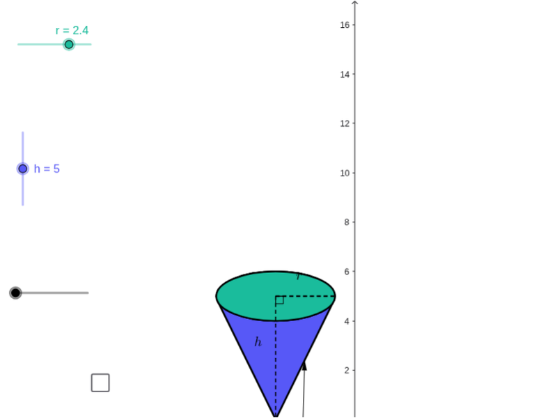
This example demonstrates how to construct a right cone and calculate its surface area using GeoGebra. Key mathematical concepts involved include the geometric properties of cones, surface area formulas, and related calculations. Construction highlights involve commands and objects such as Point, Circle, Intersect, Vector, Translate, Arc, Segment, Angle, Line, Midpoint, Conic, OrthogonalLine, Tangent, Rotate, Center, Mirror, Polygon, and CircleSector. Suitable for high school students learning solid geometry and geometric constructions.
GeoGebra Commands & Parameters
Point(xAxis) → ACircle(A, r) → cIntersect(c, xAxis) → B, CEllipse(E, D, C) → eIntersect(xAxis, yAxis) → FVector(F, G) → uTranslate(B, Vector[(u * h)]) → B'_1Translate(C, Vector[(u * h)]) → C'_1Translate(A, Vector[(u * h)]) → A'_1Translate(e, Vector[(u * h)]) → e'_1Arc(e'_1, C'_1, B'_1) → p_5Arc(e'_1, B'_1, C'_1) → qSegment(A'_1, A) → h_6Segment(A'_1, C'_1) → pAngle(A, A'_1, C'_1) → αLine(A, A'_1) → jIntersect(e'_1, j) → H, ICircle(I, r) → tIntersect(t, j, 2) → KCircle(K, I) → d_1Intersect(d_1, j, 2) → NVector(H, N) → vTranslate(H, Vector[(v * n)]) → H'_1Translate(D, Vector[(u * h)]) → D'Translate(E, Vector[(u * h)]) → E'Line(B, B'_1) → lLine(C, C'_1) → mIntersect(d_1, l, 1) → PIntersect(d_1, m, 1) → QVector(B'_1, P) → zVector(C'_1, Q) → u_1Translate(B'_1, Vector[(z * n)]) → B''Translate(C'_1, Vector[(u_1 * n)]) → C''Midpoint(B'_1, A'_1) → RMidpoint(B, A) → SLine(R, S) → a_1Intersect(q, a_1) → T,Intersect(d_1, a_1, 1) → UVector(T, U) → v_1Translate(T, Vector[(v_1 * n)]) → T'If(n ≟ 0.01, B'_1, If[n < 1, B'', P]) → B_1If(n ≟ 0.01, T, If[n < 1, T', U]) → D_1If(n ≟ 0.01, H, If[n < 1, H'_1, N]) → E_1If(n ≟ 0.01, C'_1, If[n < 1, C'', Q]) → F_1Conic(B_1, D_1, E_1, F_1, I) → g_1Conic(I, B_1, D_1, E_1, F_1) → h_1OrthogonalLine(I, j) → l_1OrthogonalLine(H, j) → b_2Intersect(m, l_1) → H_2Midpoint(H_2, C'_1) → I_2OrthogonalLine(C'_1, m) → i_2Segment(K, F_1) → m_4Translate(e, Vector[(u * h)]) → e'Tangent(A, e'_1) → a, bIntersect(e', b) → J, G_2Intersect(e', a) → L, R_2Segment(A, J) → fSegment(A, L) → gCircle(I, sqrt(h^(2) + r^(2))) → kIntersect(k, j, 1) → MCircle(M, sqrt(h^(2) + r^(2))) → sSegment(M, I) → iRotate(I, γ, M) → I'_1Rotate(I, (-γ), M) → I'_2OrthogonalLine(I'_2, i_2) → b_1Intersect(b_2, b_1) → OMidpoint(H, O) → VCircle(V, O) → c_1Vector(O, I'_2) → wCenter(g_1) → WSegment(W, F_1) → e_1Vector(H, A) → w_1Translate(H, Vector[(w_1 * (n - 1))]) → H'If(n < 1, H, If[n < 2, H', A]) → ZSegment(H, Z) → f_1Rotate(I, (-δ), M) → I'Vector(L, I') → z_1Translate(c_1, Vector[(w * (n - 2))]) → k_1Center(k_1) → A_1Intersect(k_1, j) → C_1, Q_1Rotate(C_1, (180° * (n - 2)), A_1) → G_1If(n < 2, H, If[n ≤ 3, G_1, I'_2]) → H_1Mirror(H_1, j) → I_1Translate(L, Vector[(z_1 * (n - 2))]) → L'If(n < 2, L, If[n ≤ 3, L', I']) → J_1Mirror(J_1, j) → K_1Conic(I_1, H_1, J_1, I, K_1) → p_1Vector(A, M) → i_1Translate(A, Vector[(i_1 * (n - 2))]) → A'If(n < 2, A, If[n ≤ 3, A', M]) → L_1Tangent(L_1, p_1) → j_1, m_1Intersect(p_1, m_1, 1) → M_1Intersect(p_1, j_1, 1) → N_1Polygon(L_1, M_1, N_1) → poly1, n_1, l_2, m_2Arc(p_1, N_1, M_1) → q_1Line(L_1, b_2) → r_1Intersect(p_1, r_1, 1) → O_1Intersect(p_1, r_1, 2) → P_1Arc(p_1, P_1, O_1) → s_1Polygon(L_1, O_1, I_1) → poly2, i_3, l_3, o_1Polygon(L_1, H_1, P_1) → poly3, p_2, l_4, h_2Arc(p_1, O_1, I_1) → t_1Arc(p_1, H_1, P_1) → c_2Segment(L_1, I_1) → a_2Segment(L_1, H_1) → d_2Arc(p_1, H_1, I_1) → e_2Polygon(I_1, L_1, H_1) → poly4, h_3, i_4, l_5CircleSector(M, I'_2, I'_1) → f_2CircleSector(M, I'_2, I'_1) → g_2Arc(p_1, H_1, I_1) → k_2Segment(M_1, L_1) → j_2Segment(N_1, L_1) → n_2Polygon(I_1, L_1, H_1) → poly5, h_4, i_5, l_6Arc(p_1, H_1, I_1) → q_2Polygon(J, A, L) → poly6, l_7, j_3, a_3Point(xAxis) → R_1OrthogonalLine(R_1, xAxis) → r_2Intersect(i_2, r_2) → S_1Circle(R_1, r) → s_2Intersect(s_2, xAxis) → T_1, U_1OrthogonalLine(T_1, i_2) → t_2OrthogonalLine(V_1, i_2) → b_3OrthogonalLine(W_1, i_2) → c_3Intersect(i_2, t_2) → Z_1Intersect(i_2, b_3) → A_2Intersect(i_2, c_3) → B_2OrthogonalLine(U_1, xAxis) → k_3Midpoint(g) → K_2Midpoint(f_1) → L_2Point(j) → M_2Midpoint(I_1, A') → N_2Midpoint(A', H_1) → O_2Vector(M_2, N_2) → u_2Vector(M_2, O_2) → v_2Line(M_2, r_1) → p_3Point(p_3) → P_2Vector(P_2, K_2) → z_2Vector(P_2, L_2) → u_3Segment(I_1, H_1) → q_3Intersect(k_2, q_3, 2) → S_2Vector((-0.5, 0)) → v_3Translate(P_2, v_3) → P_10Translate(M_2, v_3) → P_{11}Midpoint(W, F_1) → P_{12}Vector((0, 1.1)) → v_4Translate(P_{12}, v_3) → P_{13}Translate(P_{13}, v_4) → P_{14}Midpoint(A'_1, A) → P_{15}Translate(P_{15}, Vector[(-1, 1)]) → P_{16}
AI Drawing Prompt Reference
Draw a right cone and demonstrate its surface area calculation. Start by sketching the base circle and vertex of the cone, then rotate the base circle to generate the conical surface. Indicate the height of the cone and calculate the circumference of the base and the slant height. Using this data, draw the unfolded shape of the cone, a sector, and label its area formula. Finally, verify the correctness of the cone's surface area through geometric relationships and formulas, showcasing the properties and calculation process.
The prompt above was compiled from the original drawing commands and is for reference only.