
Study Graphs of Trigonometric Functions by Mathguru
Loading the math board and drawing, please wait…
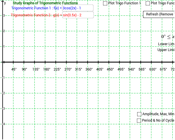
This example demonstrates how to use GeoGebra to draw and study the graphs of two trigonometric functions with upper and lower limits. Key math concepts include trigonometric functions, geometric transformations, and function graphing. Construction highlights involve commands and objects like If, Function, Derivative, RemoveUndefined, Point, Textfield, Sequence, Asymptote, Intersect, Distance, Vector, Midpoint. Suitable for high school and above students for self-study and exploration of trigonometric properties.
GeoGebra Commands & Parameters
If(angledegree, lowerlimit_d * π / 180, lowerlimit_r) → lowerlimitIf(angledegree, upperlimit_d / 180, upperlimit_r) → upperlimitFunction(g_{hidden}, lowerlimit * π, upperlimit * π) → gDerivative(g_{hidden}) → g'RemoveUndefined(Sequence[x(Root[g', i]), i, -31.41593, 31.41593, 0.31416]) → sincosturningptslistgFunction(f_{hidden}, lowerlimit * π, upperlimit * π) → fDerivative(f_{hidden}) → f'RemoveUndefined(Sequence[x(Root[f', i]), i, -31.41593, 31.41593, 0.31416]) → sincosturningptslistfPoint(g) → P_{02}Point(f) → P_{01}If(Length[sincosturningptslistg] > 0, false, true) → gchecktanfunction2Derivative(g') → g''Derivative(f') → f''If(Length[sincosturningptslistf] > 0, false, true) → fchecktanfunction1Textfield(f_{hidden}) → inputBox1Textfield(g_{hidden}) → inputBox4Sequence(Text[i + "°", (π / 180 * i - 0.05, -0.3)], i, 0, 1080, 90) → listxaxisdegreesby90If(fchecktanfunction1 ≟ false, (y(Max[f, lowerlimit * π, upperlimit * π * 10]) + y(Min[f, lowerlimit * π, upperlimit * π * 10])) / 2, meanline_{1fortan}) → meanline_1If(gchecktanfunction2 ≟ false, (y(Max[g, lowerlimit * π, upperlimit * π * 10]) + y(Min[g, lowerlimit * π, upperlimit * π * 10])) / 2, meanline_{2fortan}) → meanline_2Textfield(h_{hidden}) → inputBox5Function(h_{hidden}, lowerlimit * π, upperlimit * π) → hFunction(meanline_1, lowerlimit * π, upperlimit * π) → f_{meanline1}Function(meanline_2, lowerlimit * π, upperlimit * π) → g_{meanline2}Textfield(lowerlimit_d) → inputBox6Textfield(upperlimit_d) → inputBox7Function(0, lowerlimit * π, upperlimit * π + 1) → h_{x-axis}Textfield(upperlimit_r) → inputBox3Textfield(lowerlimit_r) → inputBox2Sequence(Text[FractionText[i] + "π", (π * i - 0.15, -0.1), true, true], i, lowerlimit + xunitdistance, upperlimit, xunitdistance) → listxaxisradianlabelSequence((i, 0), i, lowerlimit * π, upperlimit * π, xunitdistance * π) → listxaxisticksSequence(abs(f(i)), i, lowerlimit * π, upperlimit * π, 0.01) → valuestanfunctionAsymptote(f) → list5Asymptote(Function[g, lowerlimit * π, upperlimit * π]) → list6If(fchecktanfunction1 ≟ false, y(Max[f, lowerlimit * π, upperlimit * π * 10]), 0) → maxline_1If(fchecktanfunction1 ≟ false, y(Min[f, lowerlimit * π, upperlimit * π * 10]), 0) → minline_1Function(maxline_1, lowerlimit * π, upperlimit * π) → f_{maxline1}Function(minline_1, lowerlimit * π, upperlimit * π) → f_{minline1}Intersect(f_{maxline1}, vertline1) → A_1Intersect(f_{minline1}, vertline1) → B_1Intersect(f_{meanline1}, vertline1) → C_1Distance(A_1, C_1) → distanceA1C1Vector(C_1, A_1) → u_1Vector(C_1, B_1) → v_1Midpoint(A_1, C_1) → M_{A1C1}Midpoint(B_1, C_1) → M_{C1B1}If(gchecktanfunction2 ≟ false, y(Max[g, lowerlimit * π, upperlimit * π * 10]), 0) → maxline_2If(gchecktanfunction2 ≟ false, y(Min[g, lowerlimit * π, upperlimit * π * 10]), 0) → minline_2Function(maxline_2, lowerlimit * π, upperlimit * π) → g_{maxline1}Function(minline_2, lowerlimit * π, upperlimit * π) → g_{minline1}Intersect(g_{maxline1}, vertline2) → A_2Intersect(g_{minline1}, vertline2) → B_2Intersect(g_{meanline2}, vertline2) → C_2Midpoint(A_2, C_2) → M_{A2C2}Midpoint(B_2, C_2) → M_{B2C2}Distance(A_2, C_2) → distanceACVector(C_2, A_2) → u_2Vector(C_2, B_2) → v_2If(fchecktanfunction1, tancyclesf, sincoscycles1) → cycles1If(gchecktanfunction2, tancyclesg, sincoscycles2) → cycles2Intersect(g, vertline3, (0, -2)) → P_1Midpoint(P_1, Q_1) → M_{P1Q1}Vector(M_{P1Q1}, P_1) → u_{p1l}Vector(M_{P1Q1}, Q_1) → u_{p1r}Intersect(f, vertline4, (0.37243505127654164, 1.2055278889599705)) → P_2Midpoint(P_2, Q_2) → M_{P2Q2}Vector(M_{P2Q2}, Q_2) → u_{p2r}Vector(M_{P2Q2}, P_2) → u_{p2l}Derivative(f'') → f'''Derivative(g'') → g'''Sequence(Text[i + "°", (π / 180 * i - 0.15, -0.55)], i, lowerlimit * 180 + 180 * xunitdistance, upperlimit * 180, 180 * xunitdistance) → listxaxisdegreesby45
AI Drawing Prompt Reference
Draw the graphs of two trigonometric functions within specified upper and lower limits. Plot the functions and their derivatives, then identify the turning points as the roots of the derivatives. Calculate and draw the mean lines for each function, along with horizontal lines at the maximum and minimum values. Add coordinate axes, degree and radian tick marks, and asymptotes for the function graphs.
The prompt above was compiled from the original drawing commands and is for reference only.