
Study Graphs of Trigonometric Functions
Loading the math board and drawing, please wait…
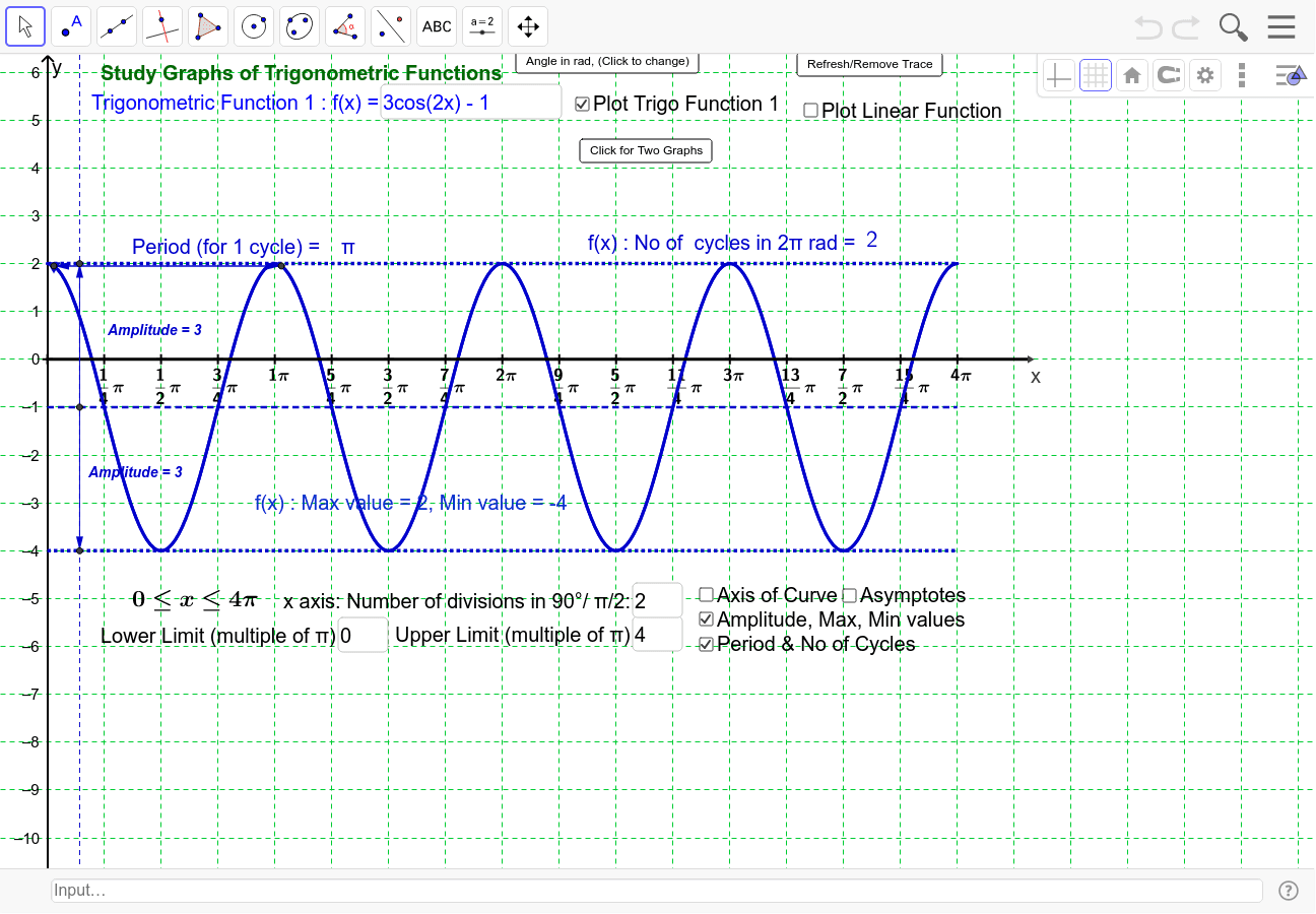
This example demonstrates how to graph and compare two trigonometric functions along with their upper and lower bounds. Key math concepts include trigonometric functions, function graphs, derivatives, and limits. It utilizes GeoGebra commands like Function, Derivative, Intersect, and Vector. Suitable for high school and above students for self-study and exploration of function properties.
GeoGebra Commands & Parameters
If(angledegree, lowerlimit_d * π / 180, lowerlimit_r) → lowerlimitIf(angledegree, upperlimit_d / 180, upperlimit_r) → upperlimitFunction(g_{hidden}, lowerlimit * π, upperlimit * π) → gDerivative(g_{hidden}) → g'RemoveUndefined(Sequence[x(Root[g', i]), i, -31.41593, 31.41593, 0.31416]) → sincosturningptslistgFunction(f_{hidden}, lowerlimit * π, upperlimit * π) → fDerivative(f_{hidden}) → f'RemoveUndefined(Sequence[x(Root[f', i]), i, -31.41593, 31.41593, 0.31416]) → sincosturningptslistfPoint(g) → P_{02}Point(f) → P_{01}If(Length[sincosturningptslistg] > 0, false, true) → gchecktanfunction2Derivative(g') → g''Derivative(f') → f''If(Length[sincosturningptslistf] > 0, false, true) → fchecktanfunction1Textfield(f_{hidden}) → inputBox1Textfield(g_{hidden}) → inputBox4Sequence(Text[i + "°", (π / 180 * i - 0.05, -0.3)], i, 0, 1080, 90) → listxaxisdegreesby90If(fchecktanfunction1 ≟ false, (y(Max[f, lowerlimit * π, upperlimit * π * 10]) + y(Min[f, lowerlimit * π, upperlimit * π * 10])) / 2, meanline_{1fortan}) → meanline_1If(gchecktanfunction2 ≟ false, (y(Max[g, lowerlimit * π, upperlimit * π * 10]) + y(Min[g, lowerlimit * π, upperlimit * π * 10])) / 2, meanline_{2fortan}) → meanline_2Textfield(h_{hidden}) → inputBox5Function(h_{hidden}, lowerlimit * π, upperlimit * π) → hFunction(meanline_1, lowerlimit * π, upperlimit * π) → f_{meanline1}Function(meanline_2, lowerlimit * π, upperlimit * π) → g_{meanline2}Textfield(lowerlimit_d) → inputBox6Textfield(upperlimit_d) → inputBox7Function(0, lowerlimit * π, upperlimit * π + 1) → h_{x-axis}Textfield(upperlimit_r) → inputBox3Textfield(lowerlimit_r) → inputBox2Sequence(Text[FractionText[i] + "π", (π * i - 0.15, -0.1), true, true], i, lowerlimit + xunitdistance, upperlimit, xunitdistance) → listxaxisradianlabelTextfield(xaxisnumdivquad) → inputBox8Sequence((i, 0), i, lowerlimit * π, upperlimit * π, xunitdistance * π) → listxaxisticksSequence(abs(f(i)), i, lowerlimit * π, upperlimit * π, 0.01) → valuestanfunctionAsymptote(f) → list5Asymptote(Function[g, lowerlimit * π, upperlimit * π]) → list6If(fchecktanfunction1 ≟ false, y(Max[f, lowerlimit * π, upperlimit * π * 10]), 0) → maxline_1If(fchecktanfunction1 ≟ false, y(Min[f, lowerlimit * π, upperlimit * π * 10]), 0) → minline_1Function(maxline_1, lowerlimit * π, upperlimit * π) → f_{maxline1}Function(minline_1, lowerlimit * π, upperlimit * π) → f_{minline1}Intersect(f_{maxline1}, vertline1) → A_1Intersect(f_{minline1}, vertline1) → B_1Intersect(f_{meanline1}, vertline1) → C_1Distance(A_1, C_1) → distanceA1C1Vector(C_1, A_1) → u_1Vector(C_1, B_1) → v_1Midpoint(A_1, C_1) → M_{A1C1}Midpoint(B_1, C_1) → M_{C1B1}If(gchecktanfunction2 ≟ false, y(Max[g, lowerlimit * π, upperlimit * π * 10]), 0) → maxline_2If(gchecktanfunction2 ≟ false, y(Min[g, lowerlimit * π, upperlimit * π * 10]), 0) → minline_2Function(maxline_2, lowerlimit * π, upperlimit * π) → g_{maxline1}Function(minline_2, lowerlimit * π, upperlimit * π) → g_{minline1}Intersect(g_{maxline1}, vertline2) → A_2Intersect(g_{minline1}, vertline2) → B_2Intersect(g_{meanline2}, vertline2) → C_2Midpoint(A_2, C_2) → M_{A2C2}Midpoint(B_2, C_2) → M_{B2C2}Distance(A_2, C_2) → distanceACVector(C_2, A_2) → u_2Vector(C_2, B_2) → v_2If(fchecktanfunction1, tancyclesf, sincoscycles1) → cycles1If(gchecktanfunction2, tancyclesg, sincoscycles2) → cycles2Intersect(g, vertline3, (0, -1.5)) → P_1Midpoint(P_1, Q_1) → M_{P1Q1}Vector(M_{P1Q1}, P_1) → u_{p1l}Vector(M_{P1Q1}, Q_1) → u_{p1r}Intersect(f, vertline4, (0.08997312945277669, 1.9515599378378266)) → P_2Midpoint(P_2, Q_2) → M_{P2Q2}Vector(M_{P2Q2}, Q_2) → u_{p2r}Vector(M_{P2Q2}, P_2) → u_{p2l}Derivative(f'') → f'''Derivative(g'') → g'''Sequence(Text[i + "°", (π / 180 * i - 0.15, -0.55)], i, lowerlimit * 180 + 180 * xunitdistance, upperlimit * 180, 180 * xunitdistance) → listxaxisdegreesby45
AI Drawing Prompt Reference
Draw two trigonometric functions along with their upper and lower bounds, showing function graphs, derivatives, and limits. First, plot the graphs of the two trigonometric functions and their upper and lower bounds. Then, calculate and plot the derivatives of these functions, marking the zeros of the derivatives. Finally, calculate and plot the mean lines of the functions, and mark the maximum and minimum values of the functions.
The prompt above was compiled from the original drawing commands and is for reference only.