
Step Through Ryan-Joiner Test
Loading the math board and drawing, please wait…
In collections
Statistics Step Through Applets
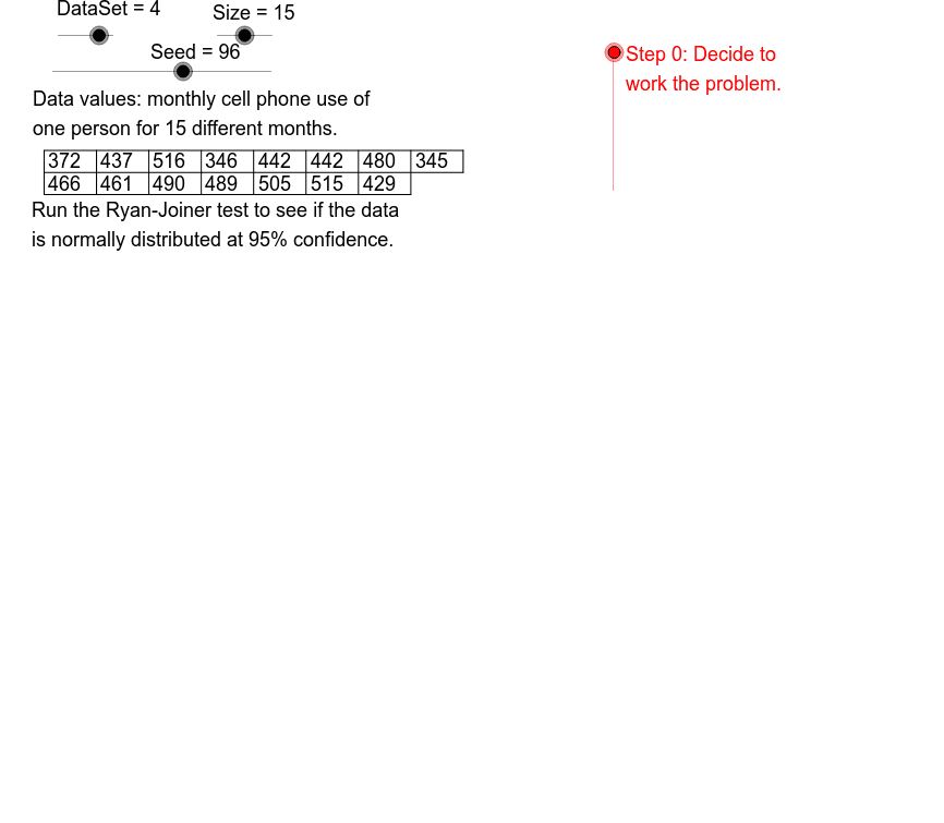
This example demonstrates the steps of the Ryan-Joiner test in statistics, showcasing its application through various examples. Key math concepts include statistical testing, probability distributions, expected value, and conditional probability. GeoGebra commands like Element, Sequence, Max, Min, KeepIf, TableText, Sort, CountIf, Segment, If, Polygon are used for data visualization and dynamic demonstrations. Suitable for high school students, university-level learners, and researchers in mathematics and statistics studying statistical methods and GeoGebra applications.
GeoGebra Commands & Parameters
Element(RateList, Mod[Seed, 8] + 1) → RateSequence(Mod[Rate * k + Start, 20] + 1, k, 0, 19, 1) → OptSeqElement(DataSets, DataSet) → DataSet1Sequence(Element[DataSet1, Element[OptSeq, k]], k, 1, Size) → DataSet2Max(DataSet2) → DataMaxMin(DataSet2) → DataMinSequence(8.5 - 1.1 * k, k, 0, 2) → LHSeqSequence(k, k, 1, 19) → StartSeqKeepIf(floor(20 / x) ≠ 20 / x, StartSeq) → RelPrimeSequence(Element[DataSet2, k], k, RL1 + 1, Size) → Data2Sequence(Element[DataSet2, k], k, 1, RL1) → Data1TableText({Data1, Data2, "hr"}) → DataListElement(DescSeq, DataSet) → DataDescTableText({DataSet2}, "hr") → DataLineSort(DataSet2) → SortDataCountIf(x > 0, RateList) → RateNoSegment(TabL1, TabR1) → HL1Segment(TabL2, TabR2) → HL2Segment(TabL0, TabR0) → HL0CountIf(x ≠ (0, 0), DataSet1) → DataCntIf(Mod[Size, 2] ≟ 1, Segment[TabR1, TabR0], Segment[TabR2, TabR0]) → DataRightSort(DataSet2) → DataSet3Sequence(Element[DataSet3, k], k, 1, RL1) → Data3Sequence(Element[DataSet3, k], k, RL1 + 1, Size) → Data4Sequence(k, k, 1, Size) → IndexSequence((k - 0.375) / (Size + 0.25), k, 1, Size) → PPVSequence(InverseNormal[0, 1, Element[PPV, k]], k, 1, Size) → InvNormSequence(k, k, 12, 18, 1) → SizeSeqSequence(" ", k, 1, 7) → SpSeqElement(CritSeq, Size - 11) → CritValPolygon((HL, HT), (HR, HT), (HR, HB), (HL, HB)) → Hilite, a, b, c, dSequence(Segment[(TL + ClWd * k, LH0), (TL + ClWd * k, LH2)], k, 0, floor(Size / 2)) → TabLinesSequence(Text[Element[Data1, k], (TL - 3.5 + k * ClWd, TT - 1.25)], k, 1, RL1) → DataRow1Sequence(Text[Element[Data2, k], (TL - 3.5 + k * ClWd, TT - 1.3 - ClHt)], k, 1, RL2) → DataRow2Sequence(Text[Element[PPV, k], (8, -7 - 1.8 * k)], k, 1, Size) → PPTxtSequence(Text[Element[Index, k], (1.3, -7 - 1.8 * k)], k, 1, Size) → IndexTxtSequence(Text[Element[DataSet3, k], (27, -7 - 1.8 * k)], k, 1, Size) → ODTxtSequence(Text[Element[InvNorm, k], (17, -7 - 1.8 * k)], k, 1, Size) → InvNormTxtSequence(Text[Element[SizeSeq, k], (38, -19 - 1.8 * k)], k, 1, 7) → SizeTxtSequence(Text[Element[CritSeq, k], (44, -19 - 1.8 * k)], k, 1, 7) → CVSeq
AI Drawing Prompt Reference
Illustrate the steps of the Ryan-Joiner test in statistics, showcasing probability distributions, expected value, and conditional probability. Use sliders to control datasets and distributions, visualizing data with bar charts and line graphs, and label key values and statistics. First, plot the datasets and distribution curves, then add sliders to adjust parameters, finally marking the maximum, minimum, and test critical values.
The prompt above was compiled from the original drawing commands and is for reference only.