
Step Through Mean & Standard Deviation of Grouped Data (TI-83/84 Simulation)
Loading the math board and drawing, please wait…
In collections
Statistics Step Through Applets
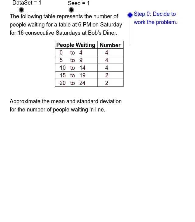
① This GeoGebra applet demonstrates step-by-step estimation of the mean and standard deviation for grouped data, simulating the workflow of a TI-83 or TI-84 calculator. ② Core mathematical concepts include arithmetic mean, standard deviation, class midpoints, frequency weighting, and cumulative frequency for grouped frequency distributions. ③ Construction highlights: uses GeoGebra commands such as Element, Sequence, Max, Min, If, Sum, Segment, Append, and Text to build the data table and step-by-step calculation panels; objects like Data, Cls0, UB, LB, CW, MdPtSq, FrqSq define class boundaries, class width, midpoints, and frequency sequences. ④ Suitable for high school or introductory college statistics courses, this applet helps students visualize the calculation process and serves as an interactive teaching or self-study tool.
GeoGebra Commands & Parameters
Element(MnSq, DataSet) → GnMnElement(RngSq, DataSet) → RngSequence(GnMn + Mod[Start + (Rate * k), Rng], k, 1, Size) → DataMax(Data) → MxDtMin(Data) → MnDtIf(CW > UB, Cls0 - 1, Cls0) → Cls1Sequence(MnDt + (k * CW), k, 0, Cls1 - 1) → LCLSequence(UCL0 + (k * CW), k, 0, Cls1 - 1) → UCLSequence("to", k, 1, Cls0) → ToSqSequence(CountIf[Element[LCL, k] ≤ x ≤ Element[UCL, k], Data], k, 1, Cls1) → FrqSqSum(FrqSq) → ChkSzSequence((Element[LCL, k] + Element[UCL, k]) / 2, k, 1, Cls1) → MdPtSqSegment(UL, UR) → tbtpSegment(UL, LL) → tblfSegment(UR, LR) → tbrtSegment(UM, LM) → tbmdSequence((Element[MdPtSq, k] * Element[FrqSq, k]), k, 1, Cls1) → XFSqSequence((Element[MdPtSq, k]^(2) * Element[FrqSq, k]), k, 1, Cls1) → XsqFSqSum(XsqFSq) → SmXsqFSum(XFSq) → SmXFElement(DDSq, DataSet) → DDElement(ClsLbSq, DataSet) → ClassElement(SbjSq, DataSet) → StatObjElement(UntSq, DataSet) → UnitAppend(FrqSq, "------") → FrqTbAppend(MdPtSq, "-----") → MdPtSqTbSequence(" ", k, 1, Cls1 + 1) → SpSqSegment(CLL, CLR) → clhzSegment(CLT, CLB) → clvrSequence("(", k, 1, Cls1) → LPrSqSequence("+", k, 1, Cls1) → PlsSqSequence(")/2 =", k, 1, Cls1) → Dv2SqIf(TbMn ≟ TbMnRd, " ", ". . .") → Dot3Segment(AH, AT) → arshftSegment(AHL, AH) → ahlSegment(AH, AHR) → ahrSequence(Segment[(TbLf, TbTp - (TbRwHt * (k + 1))), (TbRt, TbTp - (TbRwHt * (k + 1)))], k, 0, Cls1) → TbHLnSqSequence(Text[Element[FrqSq, k], (6.5, TbTp - ((k + 0.8) * TbRwHt))], k, 1, Cls1) → FrqSqTxSequence(Text[Element[UCL, k], (4.8, TbTp - ((k + 0.8) * TbRwHt))], k, 1, Cls1) → UCLTx1Sequence(Text[Element[ToSq, k], (4.2, TbTp - ((k + 0.8) * TbRwHt))], k, 1, Cls1) → ToTxSqSequence(Text[Element[LCL, k], (3.5, TbTp - ((k + 0.8) * TbRwHt))], k, 1, Cls1) → LCLTxSequence(Text["(", (0.2, TbTp - ((k + 0.8) * TbRwHt))], k, 1, Cls1) → LfPrTxSqSequence(Text[Element[LCL, k], (0.35, TbTp - ((k + 0.8) * TbRwHt))], k, 1, Cls1) → LCLTxtSequence(Text["+", (0.8, TbTp - ((k + 0.8) * TbRwHt))], k, 1, Cls1) → PlsTxSqSequence(Text[Element[UCL, k], (1.1, TbTp - ((k + 0.8) * TbRwHt))], k, 1, Cls1) → UCLTx2Sequence(Text[")/2 =", (1.5, TbTp - ((k + 0.8) * TbRwHt))], k, 1, Cls1) → RtPrTxSqSequence(Text[Element[MdPtSq, k], (2.3, TbTp - ((k + 0.8) * TbRwHt))], k, 1, Cls1) → MdSqTxSequence(Text[Element[MdPtSqTb, k], (0.5, (-1.2) - ((k + 0.9) * TbRwHt))], k, 1, Cls1) → ClMdTxText("- - - - - -", (0.5, (-1.2) - ((Cls1 + 1.9) * TbRwHt))) → Dsh1Text("- - - - - -", (2.3, (-1.2) - ((Cls1 + 1.9) * TbRwHt))) → Dsh2Sequence(Text[Element[FrqSq, k], (2.3, (-1.2) - ((k + 0.9) * TbRwHt))], k, 1, Cls1) → ClFrqTx
AI Drawing Prompt Reference
Create a statistical teaching tool to demonstrate the calculation process of mean and standard deviation for grouped data, simulating the workflow of a TI-83 or 84 calculator. Include a data table and step-by-step calculation panels showing class boundaries, widths, midpoints, and frequencies. Use sliders to control data changes, presenting data distribution and calculation results graphically for high school or introductory college statistics students.
The prompt above was compiled from the original drawing commands and is for reference only.