
Step Through Chi-Square Goodness of Fit Test
Loading the math board and drawing, please wait…
In collections
Statistics Step Through Applets
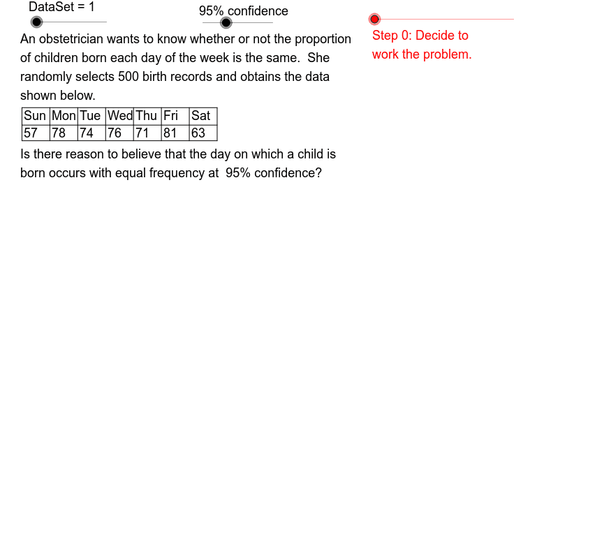
This example demonstrates the chi-square goodness of fit test process through various instances, showing how data matches theoretical distributions. Key math concepts include statistical hypothesis testing, frequency distribution, chi-square distribution, and statistical characteristics. GeoGebra commands like Element, CountIf, Sum, Sequence, If, Segment are used, along with objects such as Val1-Val6, Frq1-Frq6, DataSet. Suitable for high school students and beginners in statistics for learning hypothesis testing methods, teaching demonstrations, and data analysis practice.
GeoGebra Commands & Parameters
Element(FrqSeq, DataSet) → FrqElement(ValSeq, DataSet) → ValCountIf(x ≠ (0, 0), Frq) → KSum(Frq) → SizeElement(ConfSeq, Confidence) → ConfSequence(round(ExpVal * 100) / 100, k, 1, K) → ExpSeqSequence(Element[Frq, k] - ExpVal, k, 1, K) → OmECSequence(Element[OmEC, k]^(2), k, 1, K) → OmEsqCSequence(Element[OmEsqC, k] / ExpVal, k, 1, K) → OmEsqdECElement(OutSeq, DataSet) → OutSequence(round((Element[Frq, k] - ExpVal) * 100) / 100, k, 1, K) → OmESSequence(round(Element[OmEC, k]^(2) * 100) / 100, k, 1, K) → OmEsqSSequence(round(Element[OmEsqC, k] / ExpVal * 100) / 100, k, 1, K) → OmEsqdESIf(PVal1 ≥ 1.0E-4, PVal1, 1.0E-4) → PVal2If(PVal1 < 1.0E-4, " < ", " = ") → IE1If(PVal1 < Sig, "less than", "not less than") → RelateIf(PVal1 < Sig, "Reject", "Keep") → DecisIf(PVal1 < Sig, "IS", "IS NOT") → IOASequence(Text[Element[Frq, j], (0.2, 4.6 - 0.6 * j)], j, 1, K) → OSqTxSequence(Text[ExpVal, (1.5, 4.6 - 0.6 * j)], j, 1, K) → ESqTxSequence(Text[Element[OmES, j], (3, 4.6 - 0.6 * j)], j, 1, K) → OMESqTxSequence(Text[Element[OmEsqS, j], (4.3, 4.6 - 0.6 * j)], j, 1, K) → OMEsqSqTxSequence(Text[Element[OmEsqdES, j], (5.8, 4.6 - 0.6 * j)], j, 1, K) → OMEsqdESqTxElement(DWSq, DataSet) → DWSequence(Text[Element[Val, j], (0.3 + DW * (j - 1), 8.5)], j, 1, K) → ValSqTxSequence(Text[Element[Frq, j], (0.3 + DW * (j - 1), 8)], j, 1, K) → FrqSqTxSequence(Segment[(0.25 + k * DW, 8.85), (0.25 + k * DW, 7.9)], k, 0, K) → VrtLnSqSegment((0.25, 7.9), (0.25 + K * DW, 7.9)) → TbBtSegment((0.25, 8.35), (0.25 + K * DW, 8.35)) → TbMdSegment((0.25, 8.85), (0.25 + K * DW, 8.85)) → TbTp
AI Drawing Prompt Reference
Create a statistical chart demonstrating the chi-square goodness of fit test. Include bar charts for theoretical and actual frequency distributions, along with calculated statistics like expected values, observed values, and squared residuals. Adjust parameters using a slider to display test results under different confidence levels, with text annotations for key values. The layout should feature multiple sections showing data, calculations, and conclusions.
The prompt above was compiled from the original drawing commands and is for reference only.