Spin Cube Optical Illusion: Sinusoidal/Geometric Construction

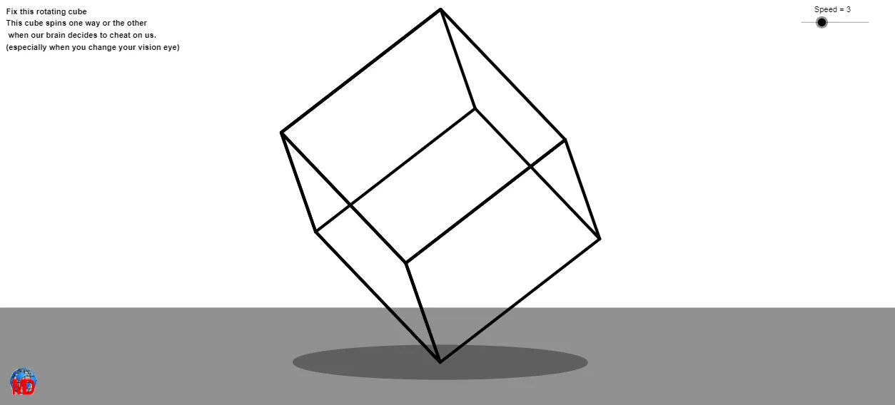
This example demonstrates an optical-illusion “spin cube” effect: from a fixed 3D viewpoint, a cube’s faces appear to rotate smoothly, creating strong depth cues. The construction is rooted in vector-based geometry and parameter-driven tracing. Key math ideas include creating and manipulating points and edges with vectors and segments, forming polygons for cube faces, computing midpoints, defining lines/rays, and finding intersections to obtain the correct projected geometry. The model also uses CurveCartesian to generate parameter-dependent curves (trajectories/positions) that support the illusion. In GeoGebra, the construction is built from commands such as Vector, Segment, Polygon, Midpoint, Line, Ray, Intersect, and CurveCartesian, along with 3D viewing via View3D and rendered face objects like poly1 and poly2. It is appropriate for upper secondary through introductory university learners, especially for lessons on solid geometry, projection effects, and the mathematical basis of optical illusions.