
Spherical Triangle: Napier's Rules
Loading the math board and drawing, please wait…
In collections
Spherical Geometry Ideas
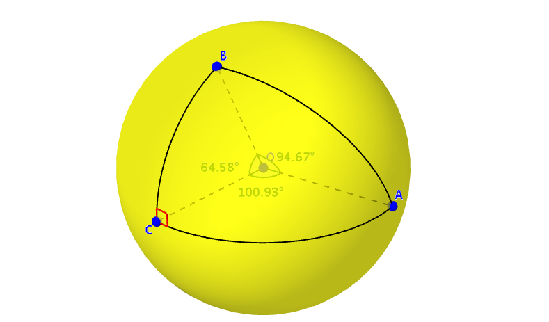
This example demonstrates the properties of spherical right triangles and the application of Napier's Rules in spherical trigonometry. Key mathematical concepts include spherical geometry, trigonometric functions, and Napier's Rules. The construction utilizes GeoGebra commands such as Sphere, Plane, IntersectPath, Intersect, Point, CurveCartesian, OrthogonalLine, Segment, OrthogonalPlane, and Angle to build the spherical right triangle and related elements. It is suitable for high school students and above, or anyone interested in understanding spherical trigonometry and its practical applications.
GeoGebra Commands & Parameters
Sphere((0, 0, 0), 1) → aPlane(zAxis, xAxis) → b_1IntersectPath(b_1, a) → cIntersect(xAxis, a, 2) → CPoint(c) → BPlane(xAxis, yAxis) → dIntersectPath(d, a) → ePoint(e) → ACurveCartesian(cos(t), 0, sin(t), t, 0, Angle[C, O, B]) → fCurveCartesian(cos(t), sin(t), 0, t, 0, Angle[C, O, A]) → bPlane(A, O, B) → hOrthogonalLine(O, h) → iPlane(B, i) → jOrthogonalLine(O, j) → kIntersect(k, a, 2) → DCurveCartesian((x(B) * cos(t)) + (x(D) * sin(t)), (y(B) * cos(t)) + (y(D) * sin(t)), (z(B) * cos(t)) + (z(D) * sin(t)), t, 0, Angle[B, O, A]) → lSegment(C, O) → mSegment(O, B) → nSegment(O, A) → pOrthogonalLine(C, m, space) → qOrthogonalPlane(C, m) → oIntersectPath(b_1, o) → rIntersectPath(d, o) → sPoint(r) → EPoint(s) → FAngle(F, C, E) → αAngle(C, O, A) → βAngle(A, O, B) → γAngle(B, O, C) → δ
AI Drawing Prompt Reference
Draw a spherical right triangle on a sphere, showing spherical geometry and trigonometric functions. Include three great circle arcs forming the triangle with a right angle at vertex C. Label the vertices A, B, C and the angles α, β, γ. Add auxiliary line segments, angle markings, and key points to illustrate Napier's Rules, with labeled planes and lines.
The prompt above was compiled from the original drawing commands and is for reference only.