
Dynamic Cone and Probability Distribution Visualization
Loading the math board and drawing, please wait…
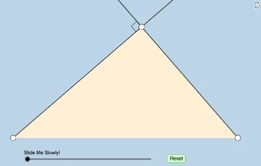
This example dynamically demonstrates the geometric relationships between a cone, unit circle, and cylinder, as well as stochastic processes and probability distributions. Key math concepts include solid geometry, trigonometry, probability & statistics, and random processes. It is constructed using GeoGebra commands like Circle, Ray, Point, Semicircle, Segment, Polygon, Midpoint, Angle, OrthogonalLine, Intersect, Rotate, Line, Distance, Dilate, Min, CircleSector, Vector, and Translate. Suitable for high school and above, ideal for geometric modeling and probability/statistics education.
GeoGebra Commands & Parameters
Circle(A, B) → cRay(A, B) → fPoint(f) → CSemicircle(A, C) → dPoint(d) → DSegment(A, D) → gSegment(D, C) → hSegment(C, A) → iPolygon(A, C, D) → t1, d_1, a, c_1Midpoint(A, C) → EAngle(A, D, C) → αOrthogonalLine(D, i) → jIntersect(j, i) → FAngle(D, F, A) → βSegment(D, F) → kAngle(D, C, F) → γAngle(F, A, D) → δRotate(F, δ / 2, A) → F'Angle(F, A, F') → εRotate(D, γ / 2, C) → D'Angle(D, C, D') → ζRay(A, F') → lRay(C, D') → mRotate(D, π / 4, F) → D'_1Angle(D, F, D'_1) → ηRay(F, D'_1) → nRotate(C, π / 4, F) → C'Angle(C, F, C') → θRay(F, C') → pIntersect(l, n) → GIntersect(m, p) → HOrthogonalLine(G, g) → qIntersect(g, q) → IOrthogonalLine(H, i) → rIntersect(i, xAxis) → JIntersect(r, i) → KLine(D, C) → sRay(G, H) → tIntersect(s, t) → LDistance(G, L) → distanceGLDistance(F, D) → distanceFDDistance(D, L) → distanceDLDistance(D, F) → distanceDFDilate(D, If[0 < b ≤ 1, 1 - b, 0], F) → D'_2Segment(D, D'_2) → eDilate(F, If[1 < b ≤ 2, 2 - b, 0], H) → F'_1Dilate(C, If[1 < b ≤ 2, 2 - b, 0], H) → C'_1Segment(F, F'_1) → f_1Segment(C, C'_1) → g_1Segment(C, L) → h_1Segment(F, K) → i_1Intersect(t, e) → MSegment(F, M) → j_1Segment(F, A) → k_1Segment(A, I) → l_1Min({h_1, i_1, j_1, k_1, l_1}) → oCircle(C, (0.7 * o)) → e_1Circle(F, (0.7 * o)) → p_1Circle(A, (0.7 * o)) → q_1Intersect(i, xAxis) → NIntersect(i, xAxis) → OIntersect(i, xAxis) → PIntersect(q_1, i) → Q,Intersect(p_1, i) → R, SIntersect(p_1, e_1) → T, , ,Intersect(e_1, s) → U, VRotate(U, If[2 < b ≤ 3, ((b - 2) * ζ), ζ], C) → U'Rotate(R, If[2 < b ≤ 3, ((b - 2) * π / 4), π / 4], F) → R'CircleSector(C, U, U') → r_1CircleSector(F, R, R') → s_1Rotate(r_1, If[4 < b ≤ 5, ((b - 4) * ζ), ζ], C) → t_1Rotate(s_1, If[4 < b ≤ 5, ((b - 4) * π / 4), π / 4], F) → c_2Dilate(A, If[5 < b ≤ 6, 6 - b, 0], G) → A'Dilate(F, If[5 < b ≤ 6, 6 - b, 0], G) → F'_2Segment(A, A') → m_1Segment(F, F'_2) → n_1Rotate(Q, If[6 < b ≤ 7, ((b - 6) * ε), ε], A) → Q'CircleSector(A, Q, Q') → d_2Rotate(d_2, If[8 < b ≤ 9, ((b - 8) * ε), ε], A) → e_2Rotate(c_2, If[8 < b ≤ 9, ((b - 8) * π / 4), π / 4], F) → f_2Dilate(G, If[9 < b ≤ 10, 10 - b, 0], H) → G'Segment(G, G') → a_1Dilate(H, If[10 < b ≤ 11, 11 - b, 0], L) → H'Segment(H, H') → b_1Dilate(D, If[11 < b ≤ 12, 12 - b, 0], L) → D'_3Angle(F, D, C) → ρRotate(D, If[13 < b ≤ 14, ((b - 13) * ρ), ρ], D) → D'_4Rotate(D'_2, If[13 < b ≤ 14, ((b - 13) * ρ), ρ], D) → WLine(G, H) → h_2Line(A, D) → i_2Line(D, C) → j_2Intersect(i_2, h_2) → ZIntersect(j_2, h_2) → A_1Dilate(G, If[10 < b ≤ 11, 11 - b, 0], Z) → G'_1Segment(G, G'_1) → k_2Dilate(F, If[11 < b ≤ 12, 12 - b, 0], Z) → F'_3Dilate(F, If[11 < b ≤ 12, 12 - b, 0], L) → F'_4Segment(F, F'_3) → g_2Segment(F, F'_4) → l_2Ray(A, D) → m_2Ray(C, D) → n_2Circle(D, 1) → p_2Intersect(p_2, n_2, 2) → B_1Angle(B_1, D, A) → ιCircle(D, (0.7 * o)) → q_2Intersect(q_2, m_2, 2) → C_1Rotate(C_1, ((-π)) / 4, D) → D_1Ray(D, D_1) → r_2Circle(D, (1.4 * o)) → s_2Intersect(s_2, r_2, 1) → E_1Rotate(C_1, If[13 < b ≤ 14, ((-(b - 13)) * π / 4), ((-π)) / 4], D) → F_1CircleSector(D, F_1, C_1) → t_2Dilate(D, If[13 < b ≤ 14, 14 - b, 0], E_1) → D'_5Segment(D, D'_5) → a_2Rotate(t_2, If[15.5 < b ≤ 16.5, ((-(b - 15.5)) * π / 4), ((-π)) / 4], D) → c_3Midpoint(D, F) → G_1Line(D, l_2) → b_2Point(m_2) → H_1Dilate(D, If[17.5 < b ≤ 18.5, 18.5 - b, 0], G_1) → D'_6Vector(D, D'_6) → uTranslate(c_3, u) → d_3Translate(D, u) → D'_7Translate(D'_5, u) → I_1Segment(D'_7, I_1) → f_3Rotate(D'_7, If[18.5 < b ≤ 19.5, ((b - 18.5) * π / 2), π / 2], G_1) → J_1Rotate(I_1, If[18.5 < b ≤ 19.5, ((b - 18.5) * π / 2), π / 2], G_1) → K_1Point(b_2) → L_1Angle(C, D, L_1) → κRotate(d_3, If[18.5 < b ≤ 19.5, ((b - 18.5) * κ), κ], G_1) → e_3Rotate(D'_7, If[18.5 < b ≤ 19.5, ((b - 18.5) * κ), κ], G_1) → M_1Rotate(I_1, If[18.5 < b ≤ 19.5, ((b - 18.5) * κ), κ], G_1) → N_1Segment(M_1, N_1) → g_3Dilate(G_1, If[19.5 < b ≤ 20.5, 20.5 - b, 0], F) → O_1Vector(G_1, O_1) → vTranslate(e_3, v) → h_3Translate(M_1, v) → P_1Translate(N_1, v) → Q_1Segment(P_1, Q_1) → i_3Dilate(D, If[20.5 < b ≤ 21.5, 21.5 - b, 0], G_1) → D'_8Vector(D, D'_8) → wTranslate(D, w) → D'_9Translate(D'_5, w) → R_1Segment(D'_9, R_1) → j_3Translate(c_3, w) → k_3Rotate(Q_1, π / 4, F) → S_1Segment(F, S_1) → l_3Line(G_1, l_3) → m_3Point(m_3) → T_1Angle(R_1, G_1, T_1) → λRotate(k_3, If[21.5 < b ≤ 22.5, ((b - 21.5) * λ), λ], G_1) → p_3Rotate(D'_9, If[21.5 < b ≤ 22.5, ((b - 21.5) * λ), λ], G_1) → U_1Rotate(R_1, If[21.5 < b ≤ 22.5, ((b - 21.5) * λ), λ], G_1) → V_1Segment(U_1, V_1) → n_3Dilate(G_1, If[22.5 < b ≤ 23.5, 23.5 - b, 0], F) → W_1Vector(G_1, W_1) → u_1Translate(p_3, u_1) → q_3Translate(U_1, u_1) → Z_1Translate(V_1, u_1) → A_2Segment(Z_1, A_2) → r_3Midpoint(D, Z) → B_2Dilate(D, If[23.5 < b ≤ 24.5, 24.5 - b, 0], B_2) → D'_{10}Vector(D, D'_{10}) → v_1Translate(c_3, v_1) → s_3Translate(D, v_1) → D'_{11}Translate(D'_5, v_1) → C_2Segment(D'_{11}, C_2) → t_3Line(B_2, g_2) → a_3Point(a_3) → D_2Angle(C_2, B_2, D_2) → μRotate(s_3, If[24.5 < b ≤ 25.5, ((b - 24.5) * μ), μ], B_2) → c_4Rotate(D'_{11}, If[24.5 < b ≤ 25.5, ((b - 24.5) * μ), μ], B_2) → E_2Rotate(C_2, If[24.5 < b ≤ 25.5, ((b - 24.5) * μ), μ], B_2) → F_2Segment(E_2, F_2) → b_3Dilate(B_2, If[25.5 < b ≤ 26.5, 26.5 - b, 0], F) → G_2Vector(B_2, G_2) → w_1Translate(c_4, w_1) → d_4Translate(E_2, w_1) → H_2Translate(F_2, w_1) → I_2Segment(H_2, I_2) → f_4
AI Drawing Prompt Reference
Visualize the dynamic relationship between a cone and a cylinder, including a unit circle and related probability distributions. Start by drawing a unit circle and a ray, then create a semicircle and a triangle based on the ray. Find the midpoint and angles, draw perpendicular lines and intersection points. Through rotation and angle calculations, create multiple new points and rays, and locate their intersections. Finally, draw line segments connecting these points and display their distance relationships to illustrate the connection between geometry and probability statistics.
The prompt above was compiled from the original drawing commands and is for reference only.