
Spherical Triangle: Napier's Rules II
Loading the math board and drawing, please wait…
In collections
Spherical Geometry Ideas
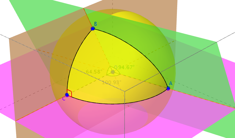
This example illustrates the application of Napier's Rules in spherical triangles. Napier's Rules are important theorems in spherical trigonometry, used to solve the relationships between sides and angles in spherical triangles. By constructing the sides and angles of a spherical triangle using GeoGebra commands such as Sphere, Plane, and IntersectPath, the example provides a visual demonstration of Napier's Rules. Suitable for high school mathematics education and students learning spherical trigonometry.
GeoGebra Commands & Parameters
Sphere((0, 0, 0), 1) → aPlane(zAxis, xAxis) → b_1IntersectPath(b_1, a) → cIntersect(xAxis, a, 2) → CPoint(c) → BPlane(xAxis, yAxis) → dIntersectPath(d, a) → ePoint(e) → ACurveCartesian(cos(t), 0, sin(t), t, 0, Angle[C, O, B]) → fCurveCartesian(cos(t), sin(t), 0, t, 0, Angle[C, O, A]) → bPlane(A, O, B) → hOrthogonalLine(O, h) → iPlane(B, i) → jOrthogonalLine(O, j) → kIntersect(k, a, 2) → DCurveCartesian((x(B) * cos(t)) + (x(D) * sin(t)), (y(B) * cos(t)) + (y(D) * sin(t)), (z(B) * cos(t)) + (z(D) * sin(t)), t, 0, Angle[B, O, A]) → lSegment(C, O) → mSegment(O, B) → nSegment(O, A) → pOrthogonalLine(C, m, space) → qOrthogonalPlane(C, m) → oIntersectPath(b_1, o) → rIntersectPath(d, o) → sPoint(r) → EPoint(s) → FAngle(F, C, E) → αAngle(C, O, A) → βAngle(A, O, B) → γAngle(B, O, C) → δIntersectPath(b_1, d) → gIntersectPath(b_1, h) → tIntersectPath(d, h) → a_1