
Spherical Coordinates (robphy) - 3D Visualization
Loading the math board and drawing, please wait…
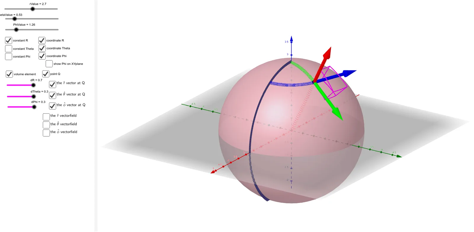
① This GeoGebra example dynamically illustrates the complete structure of spherical coordinates in 3D space, including the radial, polar, and azimuthal unit vector fields, along with grid lines and coordinate curves on a sphere. ② Core mathematical concepts include conversion between spherical and Cartesian coordinates, decomposition of 3D vectors, geometric meaning of unit vectors (r-hat, θ-hat, φ-hat), and parametric surface construction of a sphere. ③ Construction highlights: uses Surface to draw the sphere, Vector to generate vector fields in three directions, CurveCartesian for coordinate curves, Segment for reference lines; employs Zip, Flatten, Simplify for efficient list management of many vectors, and sliders (r, theta, phi) for interactive exploration. ④ Suitable for university-level calculus, multivariable functions, or vector analysis courses to teach spherical coordinates and curvilinear coordinate systems, as well as for advanced high school 3D geometry demonstrations.
GeoGebra Commands & Parameters
Simplify(sin(theta(x, y, z))) → sinThetaFlatten(Sequence[Sequence[Sequence[(i, j, k), i, (-N), N], j, (-N), N], k, (-N), N]) → gridZip(Vector[(1, 0, 0)], P, grid) → xHatsSimplify(cos(theta(x, y, z))) → rZSimplify((sinTheta(x, y, z) * sinPhi(x, y, z))) → rYSimplify((sinTheta(x, y, z) * cosPhi(x, y, z))) → rXZip(Vector[(rX(P), rY(P), rZ(P))], P, grid) → rHatsZip(Vector[P, P + If[abs(v) > maxMag, Vector[(maxMag * UnitVector[v])], Vector[v]]], P, grid, Vector[v], rHats) → fieldOFrHATSimplify(cos(theta(x, y, z))) → cosThetaZip(Vector[(thetaX(P), thetaY(P), thetaZ(P))], P, grid) → thetaHatsZip(Vector[P, P + If[abs(v) > maxMag, Vector[(maxMag * UnitVector[v])], Vector[v]]], P, grid, Vector[v], thetaHats) → fieldOFthetaHATZip(Vector[(phiX(P), phiY(P), phiZ(P))], P, grid) → phiHatsZip(Vector[P, P + If[abs(v) > maxMag, Vector[(maxMag * UnitVector[v])], Vector[v]]], P, grid, Vector[v], phiHats) → fieldOFphiHATSurface((u * cos(PhiValue)), (u * sin(PhiValue)), v, u, 0, 5, v, -5, 5) → constPhiCylVector(Q, Q + ((phiX(Q), phiY(Q), phiZ(Q)) * 2)) → QphiHatVector(Q, Q + ((rX(Q), rY(Q), rZ(Q)) * 2)) → QrHatVector(Q, Q + ((thetaX(Q), thetaY(Q), thetaZ(Q)) * 2)) → QthetaHatCurveCartesian((((rValue * sin(u)) * cos(PhiValue)), ((rValue * sin(u)) * sin(PhiValue)), (rValue * cos(u))), u, 0, ThetaValue) → ThetaVarCurveCartesian((((rValue * sin(ThetaValue)) * cos(u)), ((rValue * sin(ThetaValue)) * sin(u)), (rValue * cos(ThetaValue))), u, 0, PhiValue) → PhiVarSurface(((u * cos(PhiValue)) * sin(v)), ((u * sin(PhiValue)) * sin(v)), (u * cos(v)), u, 0, rValue + 2, v, 0, π) → constPhiRadSurface(((u * cos(v)) * sin(ThetaValue)), ((u * sin(v)) * sin(ThetaValue)), (u * cos(ThetaValue)), u, 0, rValue + 2, v, 0, (2 * π)) → constThetaCurveCartesian((((u * sin(ThetaValue)) * cos(PhiValue)), ((u * sin(ThetaValue)) * sin(PhiValue)), (u * cos(ThetaValue))), u, 0, rValue) → rVarSurface((u * sin(v)), ((u * 0) * sin(v)), (u * cos(v)), u, rValue, rValue + 0.1, v, 0, π) → zeroPhiRadFlatten(Sequence[Sequence[Sequence[(i, j, k), i, (-N), N], j, (-N), N], k, (-N), N]) → gridRECTFlatten(Sequence[Sequence[Sequence[(((r * sin((t * π / ((2 * N))))) * cos(((p * 2) * π / ((2 * N))))), ((r * sin((t * π / ((2 * N))))) * sin(((p * 2) * π / ((2 * N))))), (r * cos((t * π / ((2 * N)))))), r, 1, (2 * N)], t, 0, (2 * N)], p, 0, (2 * N)]) → gridSPHCurveCartesian((((rValue * sin(ThetaValue)) * cos(u)), ((rValue * sin(ThetaValue)) * sin(u)), 0), u, 0, PhiValue) → PhiVarXYPplaneSegment((0, 0, 0), (((rValue * sin(ThetaValue)) * cos(PhiValue)), ((rValue * sin(ThetaValue)) * sin(PhiValue)), 0)) → RadiusProjectionOnXYplaneSegment(Q, (((rValue * sin(ThetaValue)) * cos(PhiValue)), ((rValue * sin(ThetaValue)) * sin(PhiValue)), 0)) → VerticalDroppedFromQ
AI Drawing Prompt Reference
Visualize the structure of spherical coordinates in 3D space, including radial, polar, and azimuthal unit vector fields, along with grid lines and coordinate curves on a sphere. Show the sphere surface, represent unit vectors in three directions, draw coordinate curves, and add reference lines. Enable interactive exploration of radial distance, polar angle, and azimuthal angle using sliders, and illustrate the conversion between spherical and Cartesian coordinates.
The prompt above was compiled from the original drawing commands and is for reference only.