
Spherical Coordinates Brick Region Demonstration Tool
Loading the math board and drawing, please wait…
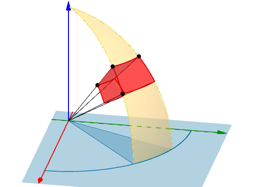
This GeoGebra demonstration tool visualizes a “brick”-shaped region in spherical coordinates, defined by the inequalities ρ₁ ≤ ρ ≤ ρ₂, φ₁ ≤ φ ≤ φ₂, and θ₁ ≤ θ ≤ θ₂. It illustrates how radial distance, polar angle, and azimuthal angle jointly bound a three-dimensional solid in space. Core mathematical concepts include spherical coordinate systems, 3D region inequalities, parametric surfaces, and coordinate transformations. The construction relies on GeoGebra commands such as Point, PointIn, If, Surface, CurveCartesian, Intersect, Segment, CircumcircleArc, and CircumcircleSector, together with objects like o, A, B, C, D, α₁, α₂, β₁, β₂, Δα, and Δβ to assemble the bounding faces, arcs, and sectors of the spherical brick. Suitable for high school advanced mathematics, university calculus, analytic geometry, and multivariable integration courses, this tool supports classroom demonstration and independent inquiry into 3D coordinate regions.
GeoGebra Commands & Parameters
PointIn(o) → AIf(x(A) > 0, atan(y(A) / x(A)), atan(y(A) / x(A)) + π) → α_1CurveCartesian((cos(α_1 + t) * sin(β_1)), (sin(α_1 + t) * sin(β_1)), cos(β_1), t, 0, 3.141592653589793) → cPoint(c) → BIf(x(B) > 0, atan(y(B) / x(B)), atan(y(B) / x(B)) + π) → α_2CurveCartesian((cos(α_1) * sin(β_1 + t)), (sin(α_1) * sin(β_1 + t)), cos(β_1 + t), t, 0, π - β_1) → dPoint(d) → CCurveCartesian((cos(α_1 + t) * sin(β_1)), (sin(α_1 + t) * sin(β_1)), cos(β_1), t, 0, Δα) → eSurface((sin(u) * cos(t)), (sin(u) * sin(t)), cos(u), u, β_1, β_2, t, α_1, α_2) → aIntersect(yAxis, zAxis) → ESegment(A, E) → fPoint(f) → FSegment(E, F) → hSegment(F, A) → iSurface(((h * sin(u)) * cos(t)), ((h * sin(u)) * sin(t)), (h * cos(u)), u, β_1, β_2, t, α_1, α_2) → bSurface(((t * sin(β_1)) * cos(u)), ((t * sin(β_1)) * sin(u)), (t * cos(β_1)), u, α_1, α_2, t, h, 1) → jSurface(((t * sin(β_2)) * cos(u)), ((t * sin(β_2)) * sin(u)), (t * cos(β_2)), u, α_1, α_2, t, h, 1) → kSurface(((t * sin(u)) * cos(α_1)), ((t * sin(u)) * sin(α_1)), (t * cos(u)), u, β_1, β_2, t, h, 1) → lSurface(((t * sin(u)) * cos(α_2)), ((t * sin(u)) * sin(α_2)), (t * cos(u)), u, β_1, β_2, t, h, 1) → mCurveCartesian((cos(α_1 + t) * sin(β_2)), (sin(α_1 + t) * sin(β_2)), cos(β_2), t, 0, Δα) → gCurveCartesian((cos(α_1) * sin(β_1 + t)), (sin(α_1) * sin(β_1 + t)), cos(β_1 + t), t, 0, Δβ) → nCurveCartesian((cos(α_2) * sin(β_1 + t)), (sin(α_2) * sin(β_1 + t)), cos(β_1 + t), t, 0, Δβ) → pSegment(B, B') → qSegment(C, C') → rSegment(D, D') → sCurveCartesian(((h * cos(α_1 + t)) * sin(β_1)), ((h * sin(α_1 + t)) * sin(β_1)), (h * cos(β_1)), t, 0, Δα) → tCurveCartesian(((h * cos(α_1 + t)) * sin(β_2)), ((h * sin(α_1 + t)) * sin(β_2)), (h * cos(β_2)), t, 0, Δα) → uCurveCartesian(((h * cos(α_1)) * sin(β_1 + t)), ((h * sin(α_1)) * sin(β_1 + t)), (h * cos(β_1 + t)), t, 0, Δβ) → vCurveCartesian(((h * cos(α_2)) * sin(β_1 + t)), ((h * sin(α_2)) * sin(β_1 + t)), (h * cos(β_1 + t)), t, 0, Δβ) → wCurveCartesian((cos(α_1 + t) * sin(β_1)), (sin(α_1 + t) * sin(β_1)), cos(β_1), t, 0, 6.283185307179586) → a_1CurveCartesian((cos(α_1 + t) * sin(β_2)), (sin(α_1 + t) * sin(β_2)), cos(β_2), t, 0, 6.28319) → b_1CurveCartesian((cos(α_1) * sin(t)), (sin(α_1) * sin(t)), cos(t), t, 0, 3.141592653589793) → c_1CurveCartesian((cos(α_2) * sin(t)), (sin(α_2) * sin(t)), cos(t), t, 0, 3.141592653589793) → d_1Segment(B, E) → f_1Segment(C, E) → g_1Segment(D, E) → h_1CircumcircleArc(H, C, G) → k_1CircumcircleArc(H, B, G) → p_1Segment(I, E) → i_1Segment(J, E) → j_1Surface((sin(u) * cos(t)), (sin(u) * sin(t)), cos(u), u, 0, β_1, t, α_1, α_2) → m_1Surface(((t * sin(u)) * cos(α_2)), ((t * sin(u)) * sin(α_2)), (t * cos(u)), u, β_1, β_2, t, 0, h) → n_1Surface(((t * sin(u)) * cos(α_2)), ((t * sin(u)) * sin(α_2)), (t * cos(u)), u, 0, β_1, t, 0, 1) → o_1Surface(((t * sin(u)) * cos(α_2)), ((t * sin(u)) * sin(α_2)), (t * cos(u)), u, β_2, 1.5707963267948966, t, 0, 1) → q_1Surface(((t * sin(u)) * cos(α_1)), ((t * sin(u)) * sin(α_1)), (t * cos(u)), u, 0, β_1, t, 0, 1) → r_1Surface(((t * sin(u)) * cos(α_1)), ((t * sin(u)) * sin(α_1)), (t * cos(u)), u, β_2, 1.5708, t, 0, 1) → s_1Surface(((t * sin(u)) * cos(α_1)), ((t * sin(u)) * sin(α_1)), (t * cos(u)), u, β_1, β_2, t, 0, h) → t_1CurveCartesian(cos(t), sin(t), 0, t, 0, 1.5707963267948966) → e_1Surface((sin(u) * cos(t)), (sin(u) * sin(t)), cos(u), u, β_2, 3.141592653589793, t, α_1, α_2) → l_1Surface((t * cos(α_1)), (t * sin(α_1)), u, t, 0, 1, u, -1, 1) → u_1Surface((t * cos(α_2)), (t * sin(α_2)), u, t, 0, 1, u, -1, 1) → v_1CircumcircleSector(I, K, J) → c_2
AI Drawing Prompt Reference
Draw a spherical‑coordinate brick region bounded by ρ₁ ≤ ρ ≤ ρ₂, φ₁ ≤ φ ≤ φ₂, and θ₁ ≤ θ ≤ θ₂. Start with the origin, then create two concentric spheres for the inner and outer radial limits. Add two cones around the z‑axis for the constant‑φ boundaries, and two half‑planes through the z‑axis for the constant‑θ boundaries. Plot the intersection curves where the spheres meet the cones and half‑planes, and draw radial segments connecting the inner and outer spheres along those curves. The six curved surfaces together enclose the solid, with visible coordinate lines showing variations in ρ, φ, and θ.
The prompt above was compiled from the original drawing commands and is for reference only.