Solving Simultaneous Linear Equations in Two Unknowns by Graphical Method

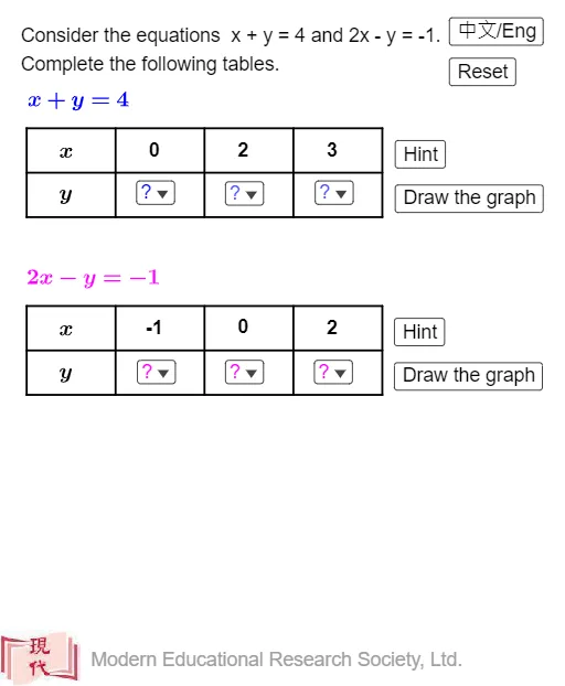
This interactive GeoGebra example demonstrates the graphical method for solving a system of two linear equations in two unknowns. The core mathematical concept is the geometric interpretation of linear systems: each equation represents a straight line in the plane, and the solution corresponds to the intersection point of the two lines. The construction uses the Line command to draw the two lines, Intersect to find their intersection point A_0, Textfield and InputBox for editable coefficients, and Sequence, Segment, and Corner to build the coordinate grid. Conditional If commands control dynamic text that indicates whether a unique solution, no solution, or infinitely many solutions exist. This resource is ideal for middle and high school students learning algebra, as well as for teachers demonstrating the connection between graphical and algebraic methods. It enhances understanding of coordinate geometry and promotes visual learning of simultaneous equations.